Cartography in R

Objectives:
1. Learn the (very) basics of map design 2. Learn how to load geospatial data
3. Learn how to inspect geospatial data
4. Plot geospatial data

Purpose

This notebook demonstrates how to work with geospatial data using the R software environment to make maps. I chose to plot the bathymetry around New Zealand. This project uses the R package marmap to querry NOAA databases to get the digital elevation model data. I then use a shapefile of the New Zealand coastlines to get better delineation between ocean and land.

Load libraries

hide

library(sf)
library(tidyverse)
library(raster)
library(here)
library(marmap)
library(ggspatial)

Load Data

Use marmap::getNOAA.bathy() to load New Zealand bathymetry and elevation data directly from NOAA database and convert bathy object to dataframe for ggplot.

hide

nz_df <- marmap::getNOAA.bathy(
  lon1 = 162,
  lon2 = 180,
  lat1 = -33,
  lat2 = -50,
  resolution = 1
) %>% 
  marmap::as.raster() %>% 
  raster::rasterToPoints() %>% 
  base::as.data.frame()%>%
              filter(layer <= 0)

Read in New Zealand coastlines with sf::read_sf() to read the shapefile containing the New Zealand coastline.

hide

nz_coast <- sf::read_sf(
    "data/nz-coastlines-and-islands-polygons-topo-150k.shp"
  )

Plot Data

Use ggplot() to plot New Zealand coastline, bathymetric raster, and depth contours.

hide

ggplot() +
  geom_raster(data = nz_df,
              aes(x = x, y = y, fill = layer)) +
  geom_contour(data = nz_df,
               aes(x = x, y = y, z = layer), color = "grey20", size = .1) +
  geom_sf(data = nz_coast,  fill = "grey40", 
          color = "black", size = .15) +
  coord_sf(xlim = c(162, 180), ylim = c(-50, -33), expand = c(0, 0)) + 
  labs(fill = "Depth (m)",
       x = "Longitude",
       y = "Latitude",
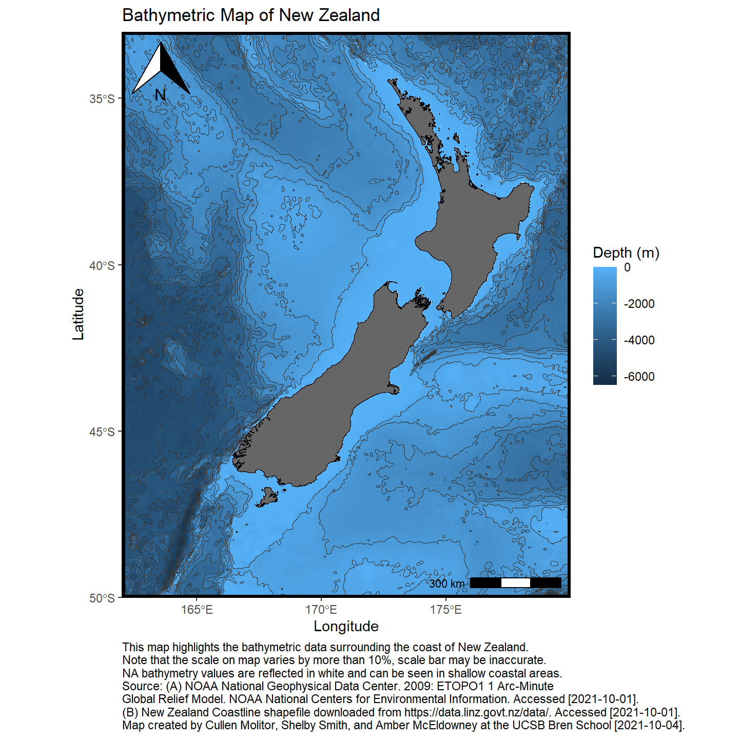
       title = "Bathymetric Map of New Zealand",
       caption = 
"This map highlights the bathymetric data surrounding the coast of New Zealand.
Note that the scale on map varies by more than 10%, scale bar may be inaccurate.
NA bathymetry values are reflected in white and can be seen in shallow coastal areas.
Source: (A) NOAA National Geophysical Data Center. 2009: ETOPO1 1 Arc-Minute 
Global Relief Model. NOAA National Centers for Environmental Information. Accessed [2021-10-01]. 
(B) New Zealand Coastline shapefile downloaded from https://data.linz.govt.nz/data/. Accessed [2021-10-01].
Map created by Cullen Molitor, Shelby Smith, and Amber McEldowney at the UCSB Bren School [2021-10-04].") +
  ggspatial::annotation_scale(location = "br") +
  ggspatial::annotation_north_arrow(which_north=TRUE, location = "tl" ) +
  theme_classic()+
  theme(panel.border = element_rect(fill = NA, size = 2, color = "black"),
        plot.caption = element_text(hjust = 0))