Import Modules

Show code

import sqlalchemy as sa
import geopandas as gpd
import pandas as pd
import matplotlib.pyplot as plt
import contextily as ctx
import math
%matplotlib inline

Database Connection

Show code

pg_uri_template = 'postgresql+psycopg2://{user}:{pwd}@{host}/{db_name}'
db_uri = pg_uri_template.format(
    drivername='postgresql+psycopg2',
    host = '{ip address}',
    user = '{username}',
    pwd = '{pwd}',
    db_name = 'osmiowa'
)
engine = sa.create_engine(db_uri)

Data Details

Database Name: - osmiowa

Database Tables: - planet_osm_line - planet_osm_point - planet_osm_polygon - planet_osm_roads - spatial_ref_sys - wind - wind_cells

Geometry: - Projected in EPSG:26975 - Geodetic CRS: NAD83 - Units: meters - Coordinate system: Cartesian 2D CS - Axes: easting, northing (X,Y) - Orientations: east, north

Query Database

Residential Scenario 1 (3H)

Show code

sql_buildings_residential_1 = \
"""
SELECT 
    ST_BUFFER(way, 450) as way
FROM 
    planet_osm_polygon 
WHERE 
    building IN ('yes', 'residential', 'apartments', 'house', 'static_caravan', 'detached')
OR 
    landuse = 'residential'
OR 
    place = 'town'
"""

Residential Scenario 2 (10H)

Show code

sql_buildings_residential_2 = \
"""
SELECT 
    ST_BUFFER(way, 1500) as way 
FROM 
    planet_osm_polygon 
WHERE 
    building 
IN 
    ('yes', 'residential', 'apartments', 'house', 'static_caravan', 'detached')
OR 
    landuse = 'residential'
OR
    place = 'town'
"""

Non-residential (3H)

Show code

sql_buildings_nonresidential = \
"""
SELECT 
    ST_BUFFER(way, 450) as way
FROM 
    planet_osm_polygon 
WHERE 
    building 
NOT IN 
    ('yes', 'residential', 'apartments', 'house', 'static_caravan', 'detached')
"""

Airports

Show code

sql_airports = \
"""
SELECT 
    ST_BUFFER(way, 7500) as way
FROM 
    planet_osm_polygon 
WHERE 
    aeroway IS NOT NULL
"""

Military Bases

Show code

sql_military = \
"""
SELECT 
    ST_BUFFER(way, 0) as way 
FROM 
    planet_osm_polygon 
WHERE 
    military IS NOT NULL
OR 
    landuse = 'military'
"""

Railways and Roads

Show code

sql_railways_n_roads = \
"""
SELECT 
    ST_BUFFER(way, 300) as way
FROM 
    planet_osm_line 
WHERE 
    (railway IS NOT NULL
     AND railway 
     NOT IN ('abandoned', 'disused', 'razed', 'dismantled'))
OR 
    (highway IS NOT NULL
AND 
    highway 
IN 
    ('motorway', 'motorway_link', 'trunk', 'trunk_link', 'road',
    'primary', 'primary_link', 'secondary', 'secondary_link'))
"""

Nature Reserves, Parks, and Wetlands

Show code

sql_nature = \
"""
SELECT 
    way 
FROM 
    planet_osm_polygon 
WHERE 
    leisure 
IN 
    ('nature_reserve', 'park')
OR
    "natural" 
IN 
    ('wetland')
"""

Rivers

Show code

sql_rivers = \
"""
SELECT 
    ST_BUFFER(way, 150) as way 
FROM 
    planet_osm_line 
WHERE 
    waterway 
IN 
    ('river')
"""

Lakes

Show code

sql_lakes = \
"""
SELECT
    way
FROM 
    planet_osm_polygon
WHERE 
    water 
IN 
    ('lake', 'reservoir', 'pond')
"""

Power Lines

Show code

sql_powerlines = \
"""
SELECT 
    ST_BUFFER(way, 300) as way
FROM 
    planet_osm_line 
WHERE 
    power IS NOT NULL
"""

Power Plants

Show code

sql_powerplants = \
"""
SELECT 
    ST_BUFFER(way, 150) as way
FROM 
    planet_osm_polygon 
WHERE 
    power IS NOT NULL
"""

Wind Turbines

Show code

sql_turbines = \
"""
SELECT
    ST_BUFFER(way, 680) as way
FROM 
    planet_osm_point 
WHERE 
    "generator:source" IS NOT NULL
AND 
    "generator:source" IN ('wind')
"""

Merge Subqueries

Scenario 1

Show code

sql_siting_constraints = \
f"""
{sql_buildings_residential_1} 
UNION
{sql_buildings_nonresidential} 
UNION
{sql_airports} 
UNION
{sql_military} 
UNION
{sql_railways_n_roads} 
UNION
{sql_nature} 
UNION
{sql_rivers} 
UNION
{sql_lakes} 
UNION
{sql_powerlines}
UNION
{sql_powerplants}
UNION
{sql_turbines}
"""
siting_constraints = gpd.read_postgis(sql_siting_constraints, con = engine, geom_col = 'way')

Scenario 2

Show code

sql_siting_constraints_2 = \
f"""
{sql_buildings_residential_2} 
UNION
{sql_buildings_nonresidential} 
UNION
{sql_airports} 
UNION
{sql_military} 
UNION
{sql_railways_n_roads} 
UNION
{sql_nature} 
UNION
{sql_rivers} 
UNION
{sql_lakes} 
UNION
{sql_powerlines}
UNION
{sql_powerplants}
UNION
{sql_turbines}
"""
siting_constraints_2 = gpd.read_postgis(sql_siting_constraints_2, con = engine, geom_col = 'way')

Show code

fig, ax = plt.subplots(figsize=(8, 8))
siting_constraints.plot(ax = ax, markersize = .1, color = "purple", alpha = .5)
ax.grid(True, color = 'dimgray')
ax.set_title('Siting Constraints (Scenario 1)', fontsize=12)
ax.ticklabel_format(scilimits =  [-5, 5])
ctx.add_basemap(ax, crs="EPSG:26975")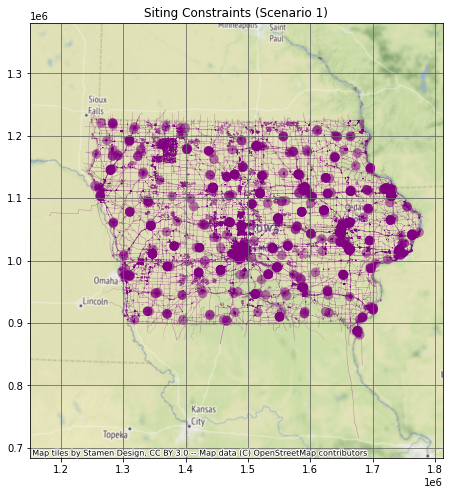

Show code

fig, ax = plt.subplots(figsize=(8, 8))
siting_constraints_2.plot(ax = ax, markersize = .1, color = "purple", alpha = .5)
ax.grid(True, color = 'dimgray')
ax.set_title('Siting Constraints (Scenario 2)', fontsize=12)
ax.ticklabel_format(scilimits =  [-5, 5])
ctx.add_basemap(ax, crs="EPSG:26975")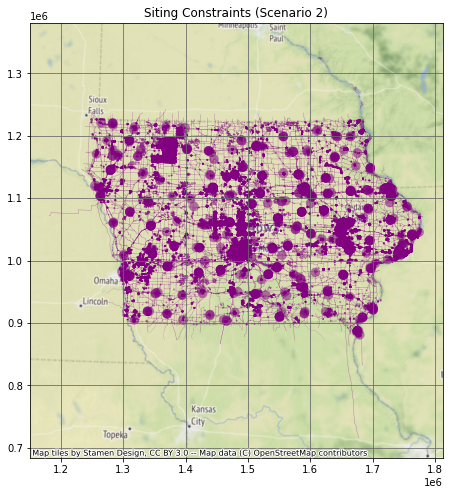

Wind Data

The table wind_cells_10000 contains 10 km2 square polygons with associated average annual wind speeds (m s-1), arranged to cover Iowa in a ragged grid.

Show code

sql_wind_speeds = \
"""
SELECT * 
FROM 
    wind_cells_10000 
WHERE 
    wind_speed IS NOT NULL
"""
wind_speeds = gpd.read_postgis(sql_wind_speeds, con = engine, geom_col = 'geom')

Results

Scenario #1

Subtract Siting Constraints from Wind Cells

Show code

suitable_cells = wind_speeds.overlay(siting_constraints, how = 'difference', keep_geom_type = False)

Plot Suitable Wind Cells

Show code

fig, ax = plt.subplots(figsize=(8, 8))
suitable_cells.plot(ax = ax, markersize = .1, color = "purple", alpha = .5)
ax.grid(True, color = 'dimgray')
ax.set_title('Suitable Areas (Scenario 1)', fontsize=12)
ax.ticklabel_format(scilimits =  [-5, 5])
ctx.add_basemap(ax, crs="EPSG:26975")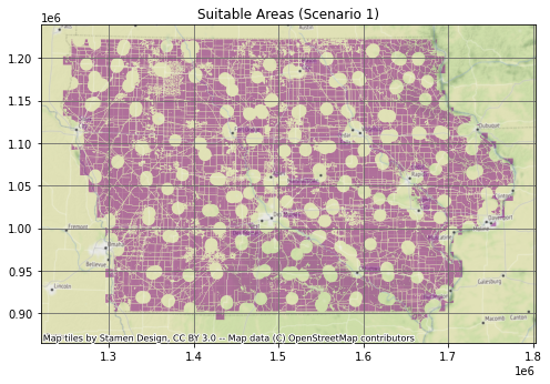

Find Number of Turbines

Show code

rotor_5x = math.pi * (136 * 5) ** 2
suitable_cells["area"] = suitable_cells['geom'].area
suitable_cells["number_wind_turbines"] = suitable_cells['geom'].area / rotor_5x

Show code

total_wind_turbines = suitable_cells["number_wind_turbines"].sum()
print("The total number of turbines in scenario 1 is:", round(total_wind_turbines))

The total number of turbines in scenario 1 is: 57286

Power production

Show code

suitable_cells['energy_per_turbine'] = 2.6 * suitable_cells['wind_speed'] - 5
suitable_cells['power_per_cell'] = suitable_cells['energy_per_turbine'] * suitable_cells['number_wind_turbines']

Total Power Production

Show code

total_scenario_1 = suitable_cells['power_per_cell'].sum()
print("The total power produced in scenario 1 is:", round(total_scenario_1), "GWH/year")

The total power produced in scenario 1 is: 1064159 GWH/year

Scenario #2

Subtract Siting Constraints from Wind Cells

Show code

suitable_cells_2 = wind_speeds.overlay(siting_constraints_2, how = 'difference', keep_geom_type = False)

Plot Suitable Wind Cells

Show code

fig, ax = plt.subplots(figsize=(8, 8))
suitable_cells_2.plot(ax = ax, markersize = .1, color = "purple", alpha = .5)
ax.grid(True, color = 'dimgray')
ax.set_title('Suitable Areas (Scenario 2)', fontsize=12)
ax.ticklabel_format(scilimits =  [-5, 5])
ctx.add_basemap(ax, crs="EPSG:26975")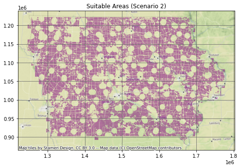

Find Number of Turbines

Show code

rotor_5x = math.pi * (136 * 5) ** 2
suitable_cells_2["area"] = suitable_cells_2['geom'].area
suitable_cells_2["number_wind_turbines"] = suitable_cells_2['geom'].area / rotor_5x

Show code

total_wind_turbines_2 = suitable_cells_2["number_wind_turbines"].sum()
print("The total number of turbines in scenario 2 is:", round(total_wind_turbines_2))

The total number of turbines in scenario 2 is: 52055

Power Production

Show code

suitable_cells_2['energy_per_turbine'] = 2.6 * suitable_cells_2['wind_speed'] - 5
suitable_cells_2['power_per_cell'] = suitable_cells_2['energy_per_turbine'] * suitable_cells_2['number_wind_turbines']
wind_speeds

	id	geom	wind_speed
0	1	POLYGON ((1256222.769 1212179.582, 1266222.769…	9.336039
1	2	POLYGON ((1266222.769 1212179.582, 1276222.769…	9.097315
2	3	POLYGON ((1276222.769 1212179.582, 1286222.769…	8.984566
3	4	POLYGON ((1286222.769 1212179.582, 1296222.769…	9.266137
4	5	POLYGON ((1296222.769 1212179.582, 1306222.769…	9.296747
…	…	…	…
1437	1438	POLYGON ((1686222.769 902179.582, 1696222.769 …	8.678687
1438	1439	POLYGON ((1426222.769 892179.582, 1436222.769 …	9.114730
1439	1440	POLYGON ((1656222.769 892179.582, 1666222.769 …	8.237385
1440	1441	POLYGON ((1666222.769 892179.582, 1676222.769 …	8.423034
1441	1442	POLYGON ((1666222.769 882179.582, 1676222.769 …	8.109468

1442 rows × 3 columns

Total Power Production

Show code

total_scenario_2 = suitable_cells_2['power_per_cell'].sum()
print("The total power produced in scenario 2 is:", round(total_scenario_2), " GWH/year")

The total power produced in scenario 2 is: 967009  GWH/year