Channel Islands SST

This notebook explores how to plot satellite sea surface temerature (SST) in the Southern California Bight around the Northern Channel Islands. This shows how to plot a static plot as well as how to animate it over time.

Libraries

hide

library(tidyverse)
library(lubridate)
library(sf)
library(rerddap)
library(marmap)
library(raster)
library(cowplot)
library(ggspatial)
library(gganimate)
library(gifski)

Geographic Data

hide

ca <- read_sf("CA.gpkg")
Site_Info <- read_csv("Site_Info.csv")

Griddap Query

hide

lat_min <- 33.35
lat_max <- 34.5
lon_min <- -120.75
lon_max <- -118.95

lat <- c(lat_min, lat_max)
lon <- c(lon_min, lon_max)

tm <- c(
  "2009-01-02T12:00:00Z",
  '2009-12-30T12:00:00Z'
)

SST <- 'jplMURSST41'
field <- 'analysed_sst'
murSST_west <- griddap(
  x = SST,
  latitude = lat,
  longitude = lon,
  time = tm,
  fields = field
)
sst <- tibble(murSST_west$data) %>%
  group_by(lat, lon) %>%
  summarise(sst = mean(analysed_sst))

Bathymetry Querry

hide

ca_bath <- marmap::getNOAA.bathy(
  lon1 = lon_min - 1,
  lon2 = lon_max + 1,
  lat1 = lat_min - 1,
  lat2 = lat_max + 1,
  resolution = 1
) %>% 
  marmap::as.raster() %>% 
  raster::rasterToPoints() %>% 
  base::as.data.frame() 

Make California Map for Inset

hide

box <- sf::st_polygon(
  x = list(
    rbind(
      c(lon_min, lat_max), 
      c(lon_max, lat_max), 
      c(lon_max, lat_min), 
      c(lon_min, lat_min),
      c(lon_min, lat_max)
    )
  )
) %>% st_sfc(crs = 4326)

C <- ggplot() +
  geom_sf(data = ca, fill = "white", size = 1) +
  geom_sf(data = box, fill = NA, size = 1, color = 'red') +
  theme_void() +
  theme(panel.border = element_rect(fill = NA),
        panel.background = element_rect(fill = alpha("white", .5)))

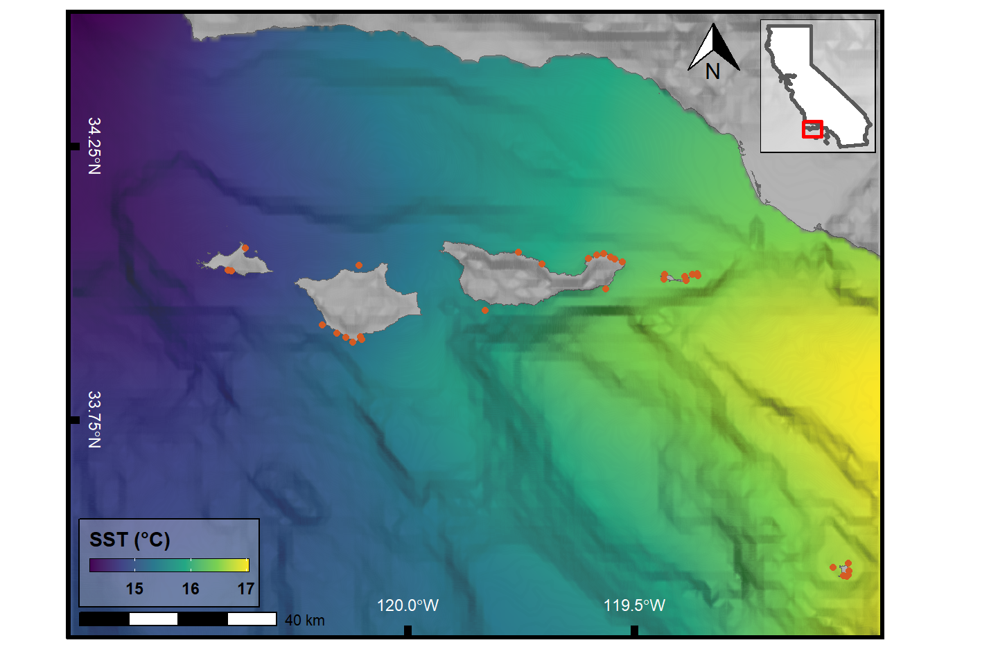
Plot Static Map

hide

main.plot <- ggplot() +
  geom_raster(data = sst, aes(x = lon, y = lat, fill = sst), interpolate = T) +
  scale_fill_viridis_c(option = 'viridis', guide = guide_colorbar(
    direction = "horizontal",frame.colour = "black",
    title.position = "top", barheight = unit(.25, 'cm'))) +
  geom_sf(data = ca, fill = "grey70", color = "grey40", size = .1) +
  geom_contour(data = ca_bath, aes(x = x, y = y, z = layer),
    breaks = seq(min(ca_bath$layer), max(ca_bath$layer), by = 5),
    color = "black", alpha = .01, size = 1) +
  scale_x_continuous(limits = lon, expand = c(0,0), breaks = c(-120, -119.5)) +
  scale_y_continuous(limits = lat, expand = c(0,0), breaks = c(33.75, 34.25)) +
  geom_point(data = Site_Info, aes(x = Longitude, y = Latitude),
             color = '#d55b23', show.legend = F, inherit.aes = F) +
  scale_color_viridis_d(option = 'magma', begin = .2, end = .8, limits = force) +
  labs(fill = "SST (\u00B0C)", x = NULL, y = NULL) +
  annotation_scale(location = "bl") +
  annotation_north_arrow(which_north = TRUE, location = "tr", pad_x = unit(2.75, "cm"),
                         height = unit(1, "cm"), width = unit(1, "cm")) +
  theme_classic() +
  theme(legend.position = c(0.125, 0.12),
        legend.title = element_text(face = 'bold'),
        legend.text = element_text(face = 'bold'),
        legend.background = element_rect(fill = alpha("white", .25), colour = 'black'),
        axis.ticks.length = unit(-0.25, "cm"),
        axis.ticks = element_line(color = "black", size = 2),
        axis.text.y = element_text(hjust = .5, margin = margin(0,-.7,0,-.5, unit = 'cm'),
                                   face = 'bold', color = "white", angle = 270),
        axis.text.x = element_text(vjust = 5, margin = margin(-0.5,0,0.5,0, unit = 'cm'),
                                   face = 'bold', color = "white"),
        panel.border = element_rect(color = "black", size = 2, fill = NA)
  )

ggdraw() +
  draw_plot(main.plot) +
  draw_plot(C, x = 0.72, y = .77, width = .2, height = .2)

Plot Animated Map

Showing 2014-2016 to highlight the 2015-2016 El Nino.

hide

redo <- FALSE

if (!file.exists("sst.gif") | redo){
  tm <- c(
    "2014-01-01T12:00:00Z",
    '2016-12-30T12:00:00Z'
  )
  
  murSST_west <- griddap(
    x = SST, 
    latitude = lat, 
    longitude = lon,
    time = tm, 
    fields = field
  )$data %>% 
    mutate(date_time = lubridate::as_datetime(time),
           date = lubridate::date(date_time)) %>% 
    group_by(date, lon, lat) %>% 
    summarise(sst = analysed_sst)
  
  p1 <- ggplot() +
    geom_raster(data = murSST_west, aes(x = lon, y = lat, fill = sst), interpolate = T) +
    scale_fill_viridis_c(option = 'viridis', guide = guide_colorbar(
      direction = "horizontal",frame.colour = "black",
      title.position = "top", barheight = unit(.25, 'cm'))) +
    geom_sf(data = ca, fill = "grey70", color = "grey40", size = .1) +
    geom_contour(data = ca_bath, aes(x = x, y = y, z = layer), 
                 breaks = seq(min(ca_bath$layer), max(ca_bath$layer), by = 5), 
                 color = "black", alpha = .01, size = 1) +
    scale_x_continuous(limits = lon, expand = c(0,0), breaks = c(-120, -119.5)) +
    scale_y_continuous(limits = lat, expand = c(0,0), breaks = c(33.75, 34.25)) +
    scale_color_viridis_d(option = 'magma', begin = .2, end = .8, limits = force) +
    labs(fill = "SST (\u00B0C)", 
         title = "{frame_time}",
         x = NULL, y = NULL) +
    annotation_scale(location = "bl") +
    annotation_north_arrow(which_north = TRUE, location = "tr", #pad_x = unit(2.75, "cm"),
                           height = unit(1, "cm"), width = unit(1, "cm")) +
    theme_classic() +
    theme(legend.position = c(0.125, 0.12),
          legend.title = element_text(face = 'bold'),
          legend.text = element_text(face = 'bold'),
          legend.background = element_rect(fill = alpha("white", .25), colour = 'black'),
          axis.ticks.length = unit(-0.25, "cm"),
          axis.ticks = element_line(color = "black", size = 2),
          axis.text.y = element_text(hjust = .5, margin = margin(0,-.7,0,-.5, unit = 'cm'),
                                     face = 'bold', color = "white", angle = 270),
          axis.text.x = element_text(vjust = 5, margin = margin(-0.5,0,0.5,0, unit = 'cm'),
                                     face = 'bold', color = "white"),
          panel.border = element_rect(color = "black", size = 2, fill = NA)) +
    gganimate::transition_time(date)
  
  gganimate::animate(p1, width = 720, height = 480,
                     # renderer = av_renderer(),
                     nframes = 100, fps = 10)
  
  anim_save(filename = "sst.gif", animation = last_animation())
}