4 Try MOSAIKS
This chapter needs testing with real users.
4.1 Overview
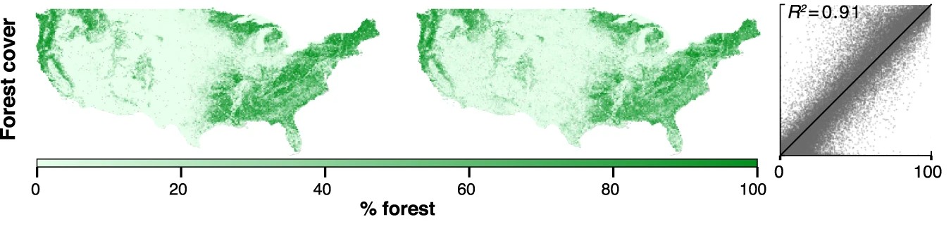
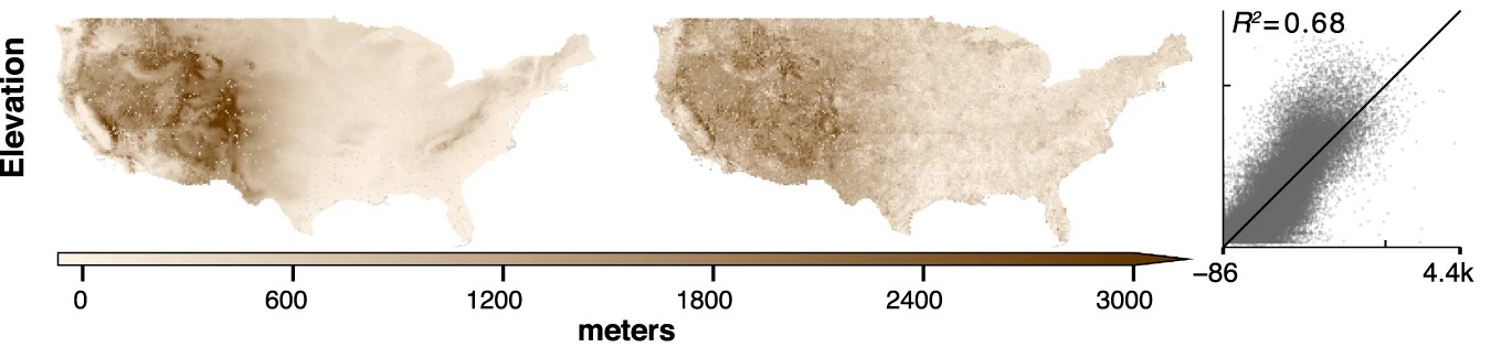
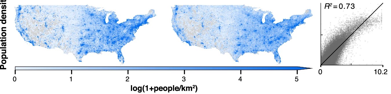
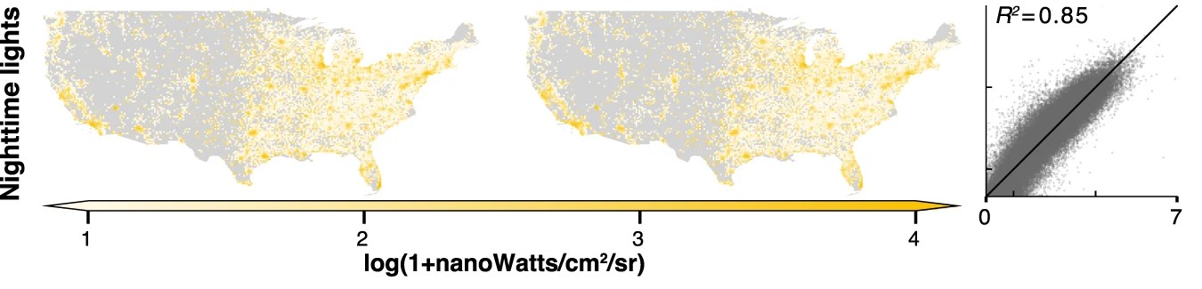
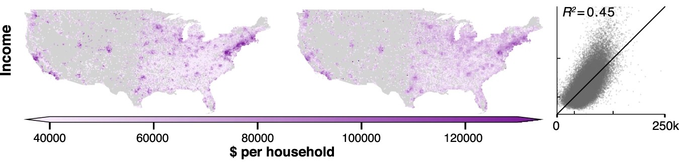
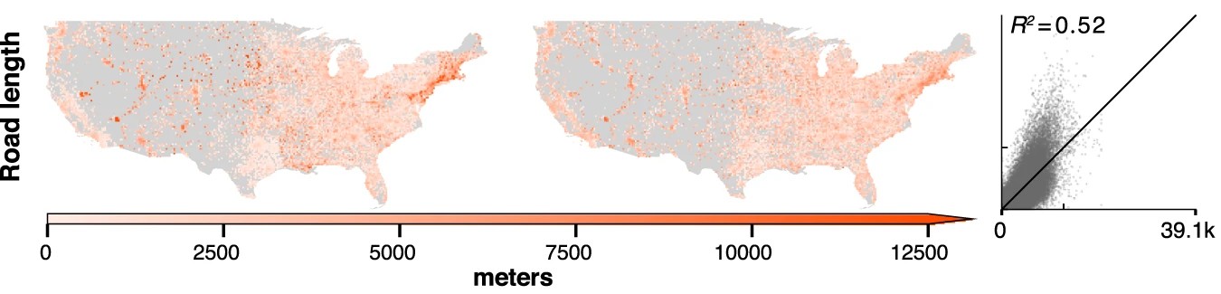
This demo replicates key results from the original MOSAIKS publication (Rolf et al. 2021). While MOSAIKS has great potential to improve access to satellite-based prediction in data-sparse environments, the original paper focused on demonstrating performance in the United States where high-quality training data was readily available.
The US served as an ideal testing ground for several reasons:
- Extensive ground truth data available across multiple variables
- Reliable spatial referencing of data
- Diverse landscapes and built environments
- Ability to benchmark against existing methods
- Systematic validation of predictions
This validation in a data-rich environment was crucial for establishing MOSAIKS as a reliable tool before deploying it in contexts where ground truth data is scarce or unreliable.
4.2 Demonstration code
4.2.1 Workflow
Below is a link to a Jupyter notebook intended to demonstrate practical use of MOSAIKS with real data. In fact, this notebook uses the original input data and features from Rolf et al. 2021. The code demonstrates:
- Loading pre-computed MOSAIKS features and labels
- Merging the features and labels
- Training a ridge regression model
- Evaluating predictions
- Visualizing results
4.2.2 Label data
The demo showcases MOSAIKS predicting several variables, and with a subset of the data used in, the original paper. The variables include:
A user simply needs to select which variable they would like to predict, and no other changes need to be made to the code. All data has been preprocessed and the code will download the necessary files from Zenodo.
4.2.3 Constraints
To stay within the Colab free tier limits of memory usage, we subset the data. We take a 50% random sample of both features (K=4,000 instead of 8,192) and observations (N=50,000 instead of 100,000) compared to the original paper. Despite using this reduced dataset, the demo still achieves strong predictive performance, highlighting MOSAIKS’s efficiency.
4.3 Run the code!
↓↓↓↓↓↓↓↓↓↓↓↓↓↓↓↓![]()
Remember to click File -> Save a copy in Drive to save any changes you make.
Or to view a static version of the code on GitHub, click the badge below.![]()
For instructions and tips on using Google Colab, please refer to Chapter 1.
4.4 Don’t want to run code?
Consider watching this demonstration instead!
4.5 What’s next?
After establishing MOSAIKS’s capabilities in the US context, the MOSAIKS development team have successfully demonstrated the system in many additional settings. This includes on the global scale, or in settings with few or low quality data. In the coming chapters, we will explore some of these applications, showing how MOSAIKS can help address data gaps in regions where traditional data collection is challenging or costly.
In the next section we will take a closer look at the label data that can be used with MOSAIKS.