16 Build, evaluate, deploy

This chapter is in early draft form and may be incomplete.

16.1 Overview

When using MOSAIKS (Multi-task Observation using SAtellite Imagery & Kitchen Sinks), model selection largely depends on your label data type. While more complex methods are certainly possible, experience shows that linear models often perform remarkably well. This is because the random convolutional features in MOSAIKS already capture and encode non-linear information from the underlying satellite imagery. This chapter will outline modeling approaches for different types of label data, and offer guidance on best practices for model evaluation.

16.2 Train/validation and test splits

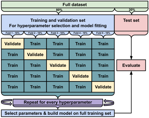
Before jumping into the details, it is important to emphasize that all modeling tasks benefit from a systematic approach to training, validation, and testing:

Train/validation split (80% of the data)
Test split (20% of the data)

This ensures that you have separate, unbiased datasets for both model tuning and final performance evaluation.

Figure 16.1: Train/validation and test splits shown for a standard 5-fold cross validation procedure.

16.3 Continuous labels

Many MOSAIKS applications involve predicting continuous outcomes such as forest cover percentage, population density, average income, crop yields, or building height. In these cases, penalized linear regression approaches (especially ridge regression) work well. These methods offer simplicity, computational efficiency, and interpretability, while mitigating overfitting through the use of regularization.

16.3.1 Ridge regression

Ridge regression (L2 regularization) is often the default choice in MOSAIKS applications because it effectively handles the large number of potentially correlated features produced by the random convolution process. It achieves this via an L2 penalty on the regression coefficients, which shrinks coefficients towards zero and reduces variance, thereby improving generalization.

The ridge regression objective function:

\[ \min_{\beta} \|y - X\beta\|^2_2 + \lambda\|\beta\|^2_2 \]

Where:

\(\lambda\) controls the strength of the regularization,
\(\beta\) are the regression coefficients,
\(y\) is the vector of observed labels,
\(X\) is the feature matrix produced by the MOSAIKS pipeline.

16.3.2 Lasso regression

Lasso regression (L1 regularization) can actually set coefficients to exactly zero, effectively performing feature selection. The L1 penalty helps enforce sparsity, which can be valuable when interpretability or identification of key features is a priority. This property makes Lasso particularly valuable when you want to identify which MOSAIKS features contribute most strongly to predictions.

The lasso objective function:

\[ \min_{\beta} \|y - X\beta\|^2_2 + \lambda\|\beta\|_1 \]

Where:

\(\lambda\) again controls the strength of the penalty,
The \(\|\beta\|_1\) term encourages some coefficients to be exactly zero.

Both can be easily implemented using scikit-learn:

from sklearn.linear_model import Ridge, Lasso

# Ridge regression
ridge = Ridge(alpha=1.0)  # alpha is the regularization strength (λ)
ridge.fit(X_train, y_train)

# Lasso regression
lasso = Lasso(alpha=1.0)
lasso.fit(X_train, y_train)

16.3.3 Why linear models work well

Though the models themselves are linear, the features are not. MOSAIKS uses random convolutions, non-linear activation functions (ReLU), and average pooling to transform raw satellite imagery into highly expressive features. Because these transformations capture a broad range of non-linear spatial patterns, traditional linear methods can then perform well with minimal additional complexity.

16.3.4 Evaluation metrics

For continuous outcomes, key evaluation metrics include:

R² (coefficient of determination): Measures the proportion of variance in the label data explained by the model.
RMSE (root mean squared error): Quantifies the average magnitude of the prediction errors.
MAE (mean absolute error): Average absolute difference between predictions and true values, less sensitive to large outliers than RMSE.

16.4 Binary classification

In some MOSAIKS applications, your labels may be binary (e.g., building presence vs. absence, land use change vs. no change). Here, logistic regression often serves as a straightforward choice.

16.4.1 Logistic regression

Logistic regression models the probability that a given example belongs to the “positive” class:

\[ \text{logit}(p) = \beta_0 + \beta_1 x_1 + \cdots + \beta_n x_n \]

where \(p\) is the probability of belonging to the positive class. Despite its simplicity, logistic regression provides robust and interpretable performance for many binary classification tasks with MOSAIKS features.

16.4.2 Evaluation metrics

For binary classification, common metrics include:

AUC-ROC: The area under the ROC curve, assessing the trade-off between true positive rate and false positive rate across different threshold settings.
Accuracy: The proportion of correct predictions.
Precision: Of the positive predictions made, how many were correct?
Recall: Of the actual positives in the dataset, how many did we correctly identify?
F1 score: The harmonic mean of precision and recall, often used in imbalanced classification settings.

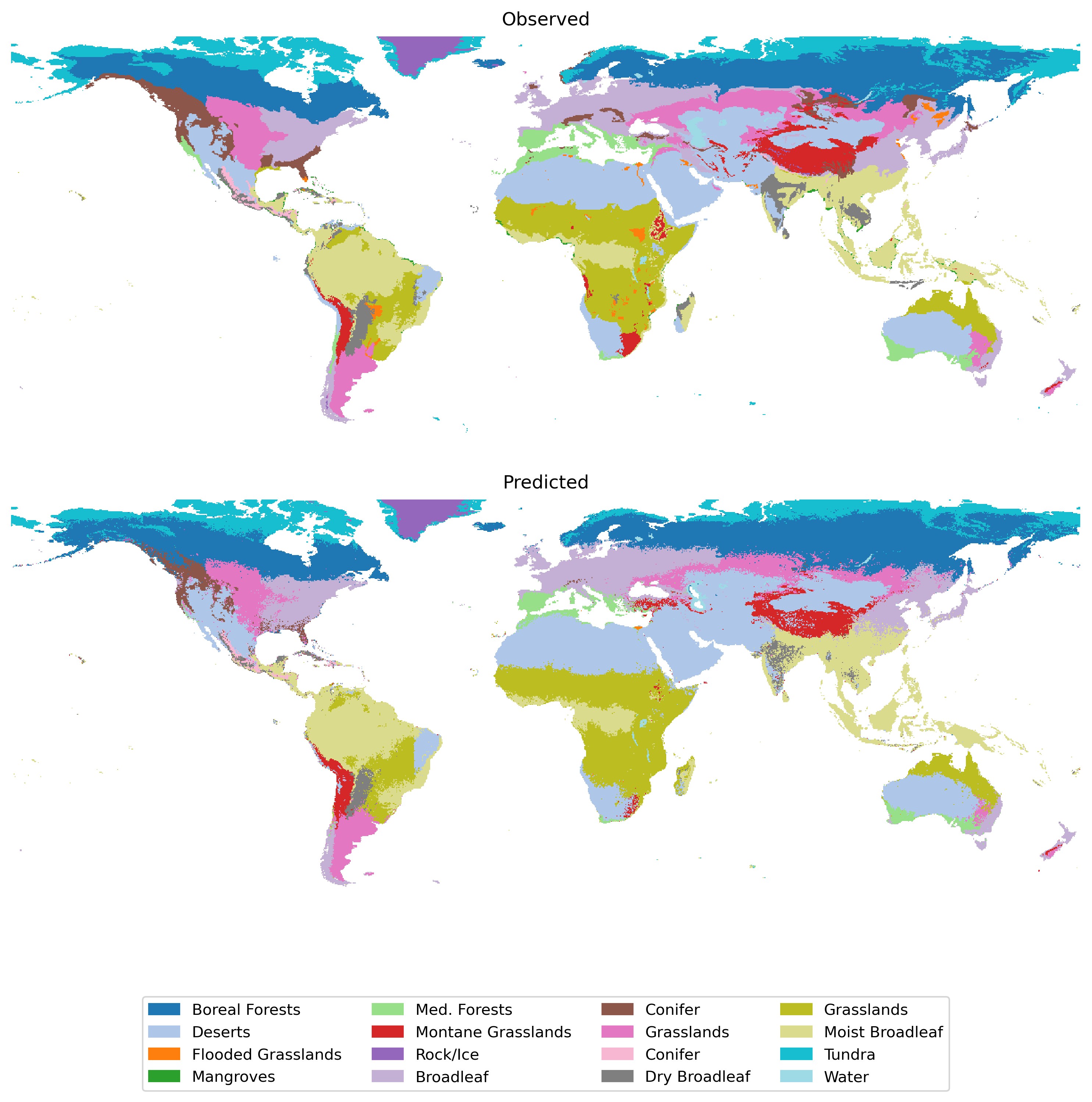
16.5 Multi-class classification

Some applications require predicting multiple categories (e.g., land cover types, crop variety, building categories). These are multi-class classification problems. Several approaches are possible:

One-vs-Rest: Train a binary classifier for each class; each classifier distinguishes one class from “all others.”
Multinomial (softmax) regression: A single model to predict probabilities across all classes simultaneously.
Ordinal regression: For predicting ordered categories (e.g., mild, moderate, severe damage).

Figure 16.2: Example of multiclass classification

16.5.1 Evaluation metrics

For multi-class problems, consider:

Overall accuracy: Percentage of examples correctly classified.
Per-class accuracy: Accuracy within each class, useful if class sizes are imbalanced.
Confusion matrix: Provides a detailed breakdown of predictions vs. actual classes.
Weighted F1 score: Averages F1 across classes, weighting by class frequency.
Cohen’s kappa: Measures agreement between predicted and actual labels, adjusting for chance agreement.

16.6 Applying the model to make predictions

Once you have selected a model and tuned it (e.g., via cross-validation), you can apply the model to new, unseen data. This step is often referred to as “inference” or “scoring”:

Prepare features: The features for the new areas or times should be extracted using the same RCF model that was used to extract the original features. This means that a model made with custom made could not be able to features on the API. The features may be randomly created, but after the model is initialized, the weights are fixed.
Load the trained model: Ensure the model (along with any hyperparameters and preprocessing steps) is loaded exactly as it was trained. This consistency is critical for maintaining predictive accuracy.
Predict: Pass the new feature matrix (X_new) into the trained model’s predict method to obtain predictions. For example, using scikit-learn:
```
y_pred = ridge.predict(X_new)
```
If your task is classification, use predict_proba to get predicted probabilities:
```
p_pred = logistic_regression.predict_proba(X_new)
```
Interpret and store results: Save the predictions in a structured format (e.g., CSV, GeoTIFF) for downstream analysis. Consider including metadata about the date and version of your model, the MOSAIKS feature extraction process, and any relevant notes on data quality.

By following these steps, you ensure that your MOSAIKS models are deployed effectively and consistently. From here, you can visualize the predictions, integrate them into downstream analyses, or inform policy and decision-making based on the model’s output.

16.6.1 Addressing domain shift

When applying your model to new geographic regions or under different conditions, be aware that the underlying data distribution (satellite imagery patterns, socioeconomic factors, land-use/land-cover types) may differ from your training set. This “domain shift” can lead to reduced predictive performance if the model has not been exposed to similar examples during training. To mitigate this, consider collecting additional representative training data from these new regions, adopting transfer learning or domain adaptation techniques, and quantifying predictive uncertainty so you can flag areas where the model may perform poorly. Periodic performance audits and retraining—especially when new data becomes available—help ensure robust generalization across diverse geographies.

Predicting at higher resolution than the labels

16.7 Quantifying uncertainty

16.8 Model selection workflow

Identify label type
- Continuous → Ridge or Lasso regression
- Binary → Logistic regression
- Multi-class → One-vs-Rest or Multinomial
Cross-validation
- Split data into train, validation, and test sets, respecting spatial structure where possible (e.g., leave-cluster-out).
- Select appropriate evaluation metrics (e.g., R² for continuous, ROC-AUC for binary).
- Tune hyperparameters (\(\lambda\) in ridge/lasso, regularization in logistic) using the validation set.
Model deployment
- Retrain on the entire training set using the chosen hyperparameters.
- Generate predictions on the test set (or new data).
- Quantify uncertainty (e.g., confidence intervals, out-of-sample error estimates).

16.9 Summary

Start with simple linear models: Let MOSAIKS features do the heavy lifting of extracting non-linear patterns.
Match the metric to the task: R² or RMSE for continuous labels, AUC-ROC or F1 score for classification, etc.
Use cross-validation: Always separate training and testing to maintain unbiased estimates of model performance.
Consider spatial structure: When dealing with spatial data, standard random splits may lead to overly optimistic estimates of performance.

The key elements for successful model building include:

Algorithm Selection
- Choose based on label type
- Consider computational needs
- Balance complexity vs performance
Cross Validation
- Use spatial awareness in splits
- Select appropriate metrics
- Tune model parameters
Model Evaluation
- Test out-of-sample performance
- Validate across space
- Quantify uncertainties
Deployment
- Train final model
- Generate predictions
- Document process
- Monitor performance

Looking forward

In the next chapter, we’ll discuss strategies for accounting for spatial dependencies in your modeling workflow, including methods for spatially stratified cross-validation, spatial interpolation, and spatial extrapolation.