12 Understanding features – MOSAIKS Training Manual

12.1 Kitchen sinks?

MOSAIKS stands for Multi-task Observation using SAtellite Imagery & Kitchen Sinks. Whenever we present MOSAIKS, we get the question, “Where does ‘kitchen sinks’ come from?” The answer stems from the phrase “everything but the kitchen sink,” which means “almost everything imaginable.” In the context of MOSAIKS, everything but the kitchen sink emphasizes that we take a huge amount of information out of the raw imagery—though, of course, we’re not capturing every last pixel or every possible relationship. It’s as if we’re taking the most useful “ingredients” (i.e., features) from the imagery and leaving the rest behind.

Figure 12.1: Maddy (Madagascar; center) takes raw satellite images (left) and uses the kitchen sink method to produce random convolutional features (right). Art by Grace Lewin.

This idea of leaving behind the raw imagery is key to MOSAIKS’s power. It means that most users never have to handle the massive amounts of satellite imagery directly. Instead, the MOSAIKS team takes on that burden—extracting a large set of random convolutional features—and then discards the imagery. End users do not need to see the raw imagery or interpret what each individual feature means; they can just use the numerical representation. As a result, users can simply download these features and apply them to their own predictive tasks.

In this section, however, we lift the hood to see what’s going on. We focus on how we extract the features from satellite imagery and attempt to provide some intuition for what these features represent.

In this book, the terms random convolutional features, RCFs, features, satellite features, and MOSAIKS features are used interchangeably.

12.2 Turning images into features

Figure 12.2: A collection of satellite images. Source: Microsoft Planetary Computer

12.2.1 Overview

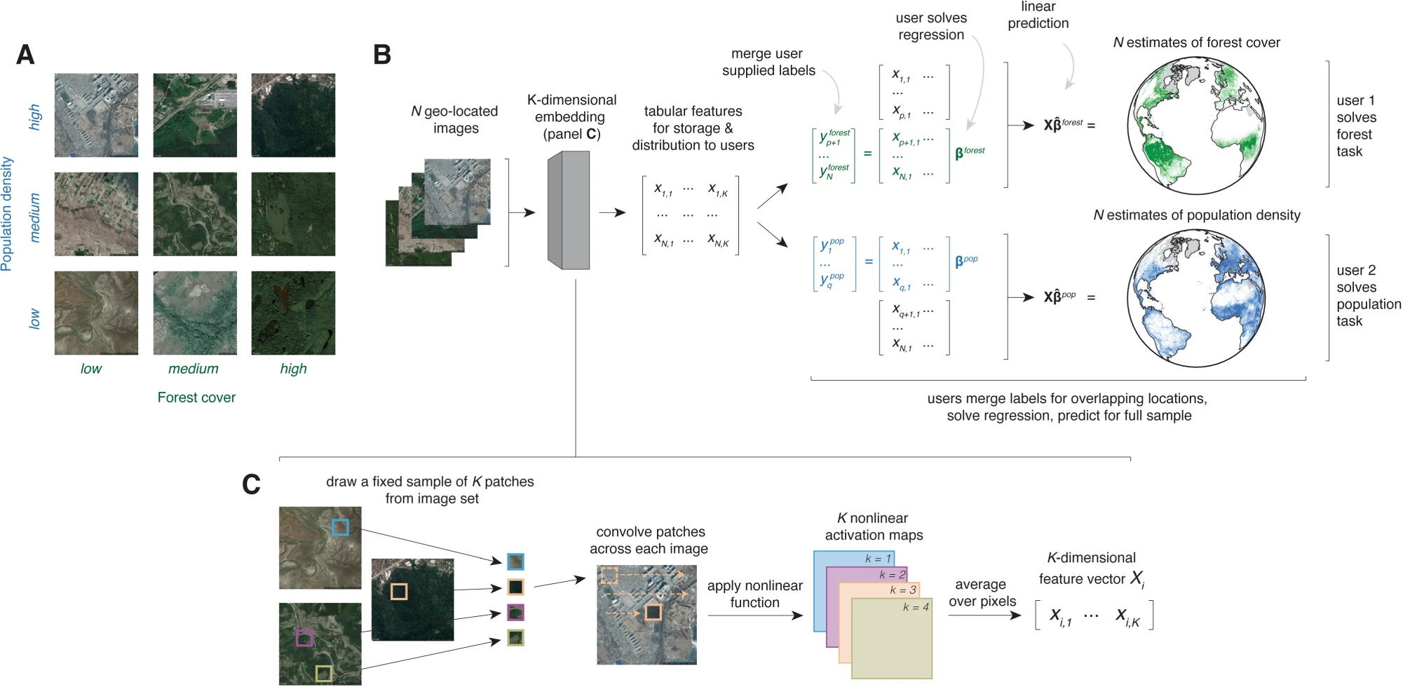
The MOSAIKS featurization process produces a fixed-length feature representation for each patch of satellite imagery. Practically, this means we end up with a numerical vector for each image. Because MOSAIKS uses satellite image, you can substitute the word image for location which means we end up with a numerical representation for each location.

Figure 12.3: A closer look at the RCF processing. Illustration of the one-time unsupervised computation of random convolutional features. K patches are randomly sampled from across the N images. Each patch is convolved over each image, generating a nonlinear activation map for each patch. Activation maps are averaged over pixels to generate a single K-dimensional feature vector for each image. Source: Rolf et al. 2021 Figure 1 C

The featurization process has three main steps: convolution, activation, and average pooling.

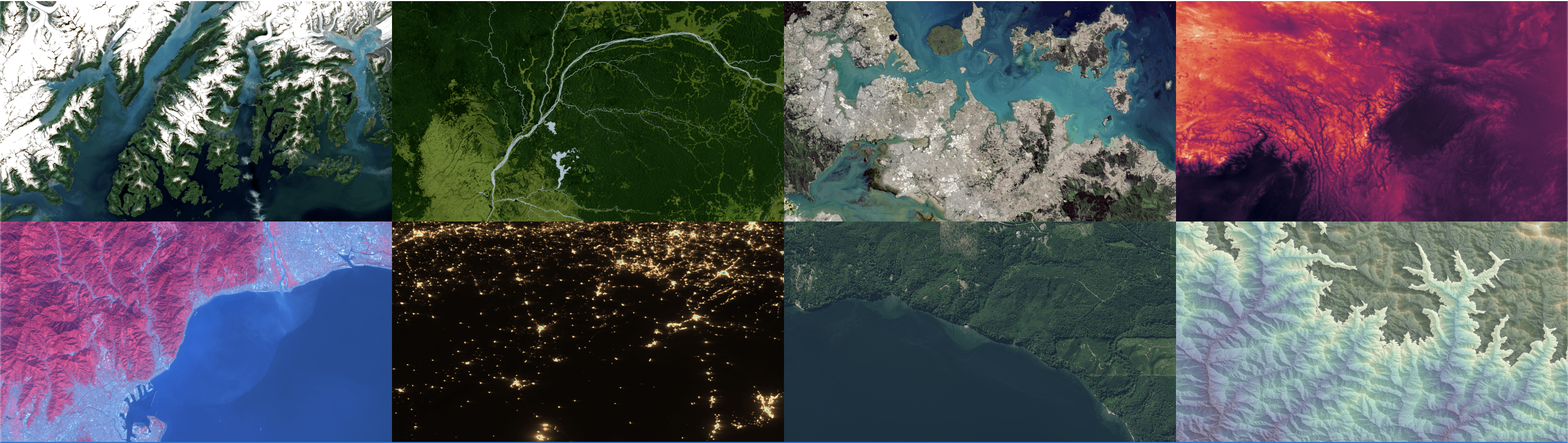
In the coming sub-sections, we will illustrate these steps. In our example, our input imagery will have the dimensions \(3 x 256 x 256\), where \(3\) is the number of color channels (red, green, and blue) and \(256 x 256\) is the image size (width x height) in pixels.

12.2.2 Understanding convolutions

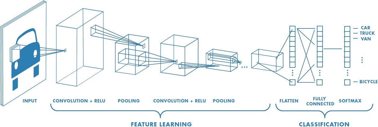
In simple terms, applying a convolution to an image can highlight certain patterns, like edges, textures, or colors. Convolutional filters “scan” across the image, computing element-wise products with small patches of the image. Many computer vision models stack multiple convolutional and other layers into a convolutional neural network (CNN). Deep neural networks can have many layers, which is why the approach is often called deep learning.

Figure 12.4: A gif showing a convolutional layer with no padding and no strides. Source: A guide to convolution arithmetic for deep learning.

MOSAIKS, on the other hand, uses a single convolutional layer. These layer weights are randomly initialized and remain fixed; they aren’t updated during training. This is why the features we get are essentially “random samples” of the spatial and spectral information in the images.

There are many great resources for visualizing convolutions, including Convolutional Neural Networks (CNNs) explained.

12.2.2.1 Initializing filters

For the convolution step, we need to initialize a set of filters. Each filter is a 3-dimensional tensor with the same number of color channels as the images and a width and height size specified by a kernel size parameter. We can initialize these filters in two ways:

Gaussian initialization: We draw the filter weights from a normal distribution.
Empirical patches: We randomly sample patches from the image dataset and use these as filters.

Either way, each filter has the same number of color channels as the original images and a specified kernel size (e.g., 3×3). So if our kernel size is 3, each filter might have shape (3, 3, 3). The number of filters is a hyperparameter that you can set when you define your model.

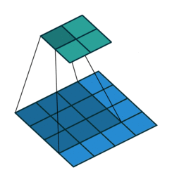
To perform the convolution, we compute the dot product of each filter with every portion of the image as the filter slides across it. The result is a new image (a convolution output map) that highlights regions similar to that filter’s pattern.

We use pytorch’s torch.nn.functional.conv2d function to perform this operation.

12.2.2.2 Whitening filters

If you decide to use empirical patches in the convolution step, it is best practice to whiten the patches. We use a process called Zero-phase Component Analysis (ZCA) whitening, which preserves the spatial structure of the data while removing correlations among pixels.

The key steps are:

Subtract the mean of each feature from the data.
Compute the covariance matrix \(\Sigma\) and perform its eigendecomposition.
Use the eigenvectors \(U\) and eigenvalues \(D\), along with a small constant \(\varepsilon\), to form the ZCA transform \(W\).
Multiply the original data by \(W\) to obtain the whitened data \(\widetilde{X}\).

Mathematically, assuming \(X\) is your zero-mean data matrix of shape \((N \times d)\):

\[ \Sigma = \frac{1}{N} X^\top X \quad\quad\text{and}\quad\quad \Sigma = U \, D \, U^\top, \]

\[ W = U \Bigl(D + \varepsilon I\Bigr)^{-\tfrac{1}{2}} U^\top, \]

\[ \widetilde{X} = X \, W. \]

See the ZCA whitening implementation in torchgeo for more details.

12.2.3 Activation

Next, we apply a non-linear activation function—ReLU (Rectified Linear Unit)—to the convolution output map. ReLU outputs max(0, x), meaning it zeroes out negative values. This step helps capture non-linearities in the data.

The 2-for-1 activation special

When we define our model, one of the parameters that needs to be specified is the number of features. This number needs to be a positive value because we generate 2 features for each filter.

We do this by applying the activation function twice:

Feature A – ReLU activation on the convolution output.
Feature B – ReLU activation on the inverted convolution output (i.e., multiplication by –1, or “negative” of the same filter output).

So if you specify 200 features, you are actually drawing 100 weights and getting 200 features back. This improves computational efficiency and ensures that each filter has the potential to capture both positive and negative cues.

12.2.4 Average pooling

We then apply an adaptive average pooling layer to each activation map, collapsing the 2D spatial grid into a single number per filter. Essentially, this “global average” is a single summary value for how strongly that filter responded to the image.

We use pytorch’s torch.nn.functional.adaptive_avg_pool2d function to perform this operation.

12.2.5 Putting it all together

We repeat the 3 steps (convolution, activation, and pooling) for all filters. If we have K filters, we end up with a K-dimensional feature vector.

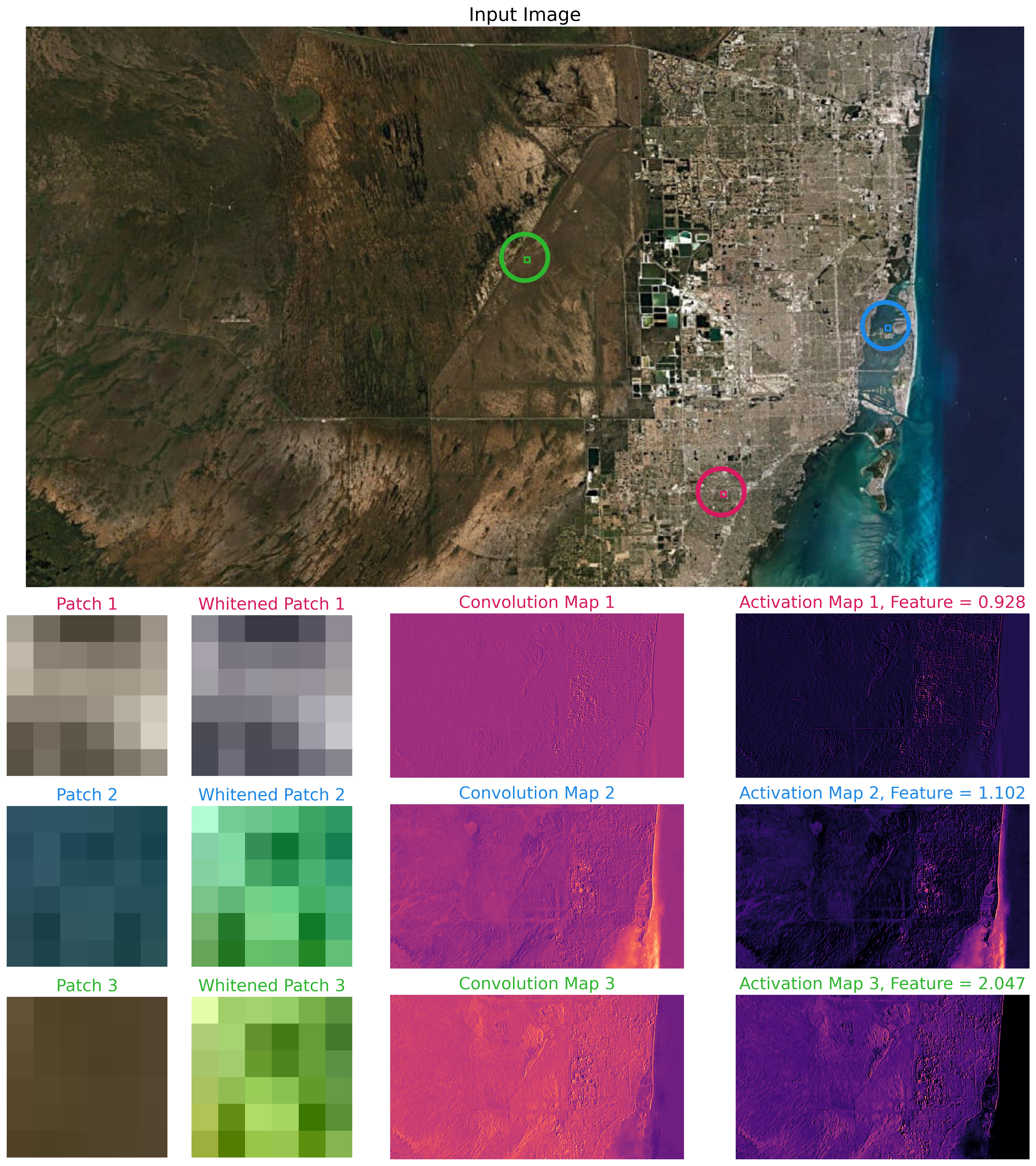
Figure 12.5: Input image, selected patches, whitened patches, convolution output, and activation maps

12.3 Intuition for RCFs

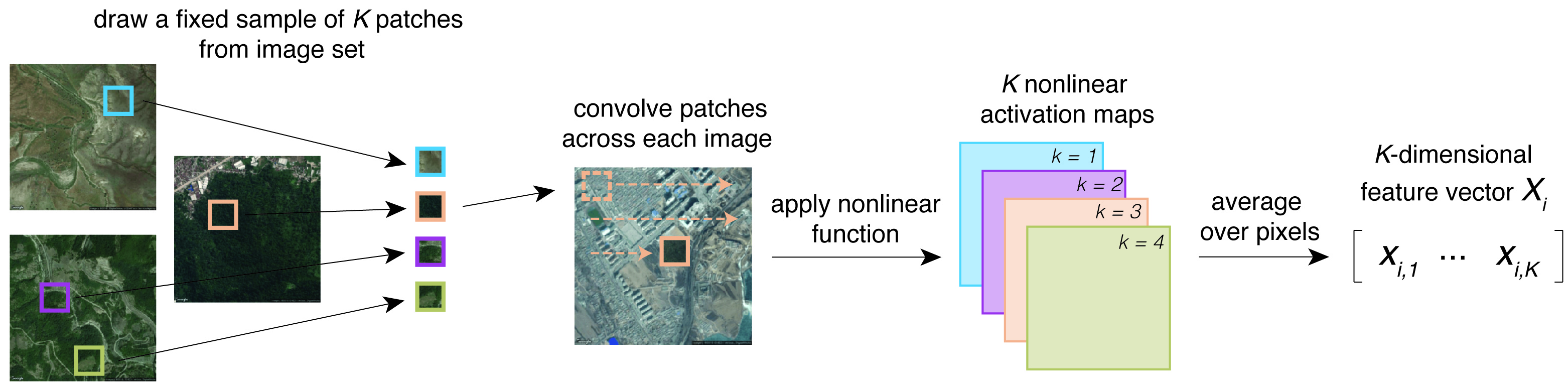
Below is a cartoon that illustrates what a random convolutional feature vector might be looking for. Suppose we randomly draw three 3×3 patches from different parts of an image: a forest patch, a road patch, and a river patch.

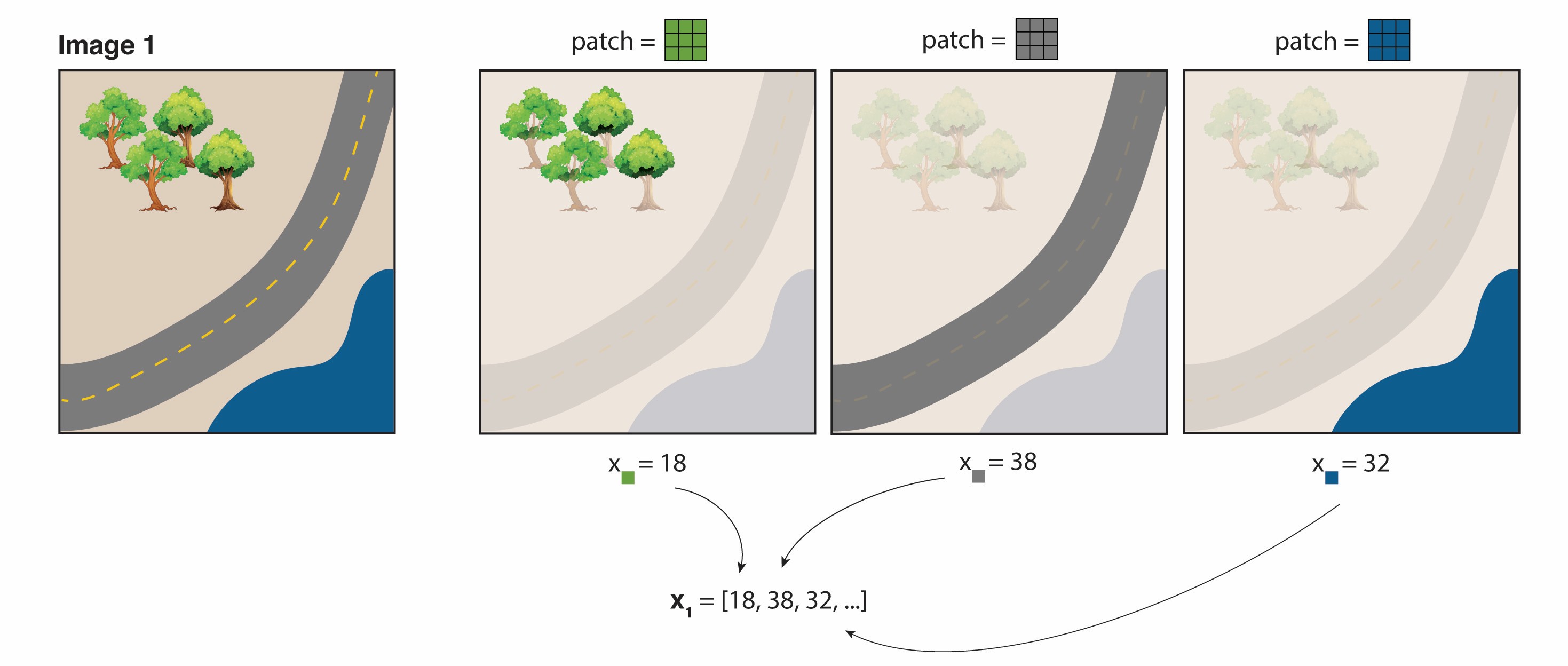
Figure 12.6: A single image with 3 random convolutional patches, highlighting 3 different feature activations of the imagery.

When we convolve the forest patch across the entire image, the resulting map “lights up” places that look like forest. Likewise, the road patch lights up roads, and the river patch lights up the river. After the ReLU and average-pooling steps, we get a set of summary values—one for each filter.

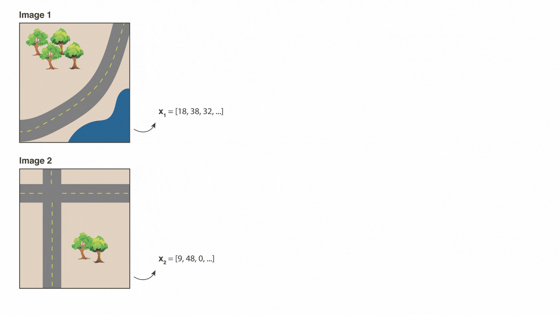
Figure 12.7: Two cartoon images with the same patches used in the convolution step. We see that we have several labels for each image and that we can model each outcome with the same set of features.

If Image 1 has more trees than Image 2, the “forest” feature’s value is higher in Image 1. If Image 2 has more roads, its “road” feature will be higher. Because these features each capture a different (random) spatial pattern, we can then combine them for many downstream prediction tasks—whether it’s predicting tree cover, paved roads, or even something else that correlates with these visual patterns.

Figure 12.8: A cartoon image projected into random feature space. If we look at just 2 dimensions, how grey on the x-axis and how green on the y-axis, we can find the vector through this feature space which represents our outcome.

12.4 Why use RCFs?

12.4.1 Traditional convolutional neural networks (CNNs)

To appreciate RCFs, let’s contrast them with traditional CNNs. In a standard CNN, filters are learned via backpropagation. The network sees many examples, calculates errors, and updates the filter weights so that over time they become good at extracting task-specific features. This makes CNNs powerful, but only for what they have been trained to do.

Figure 12.9: A simplified diagram showing a typical convolutional neural network model architecture.

12.4.2 Replacing minimization with randomization in learning

MOSAIKS takes a radically simpler approach: random filters are used to sample the imagery’s information. Because they are random, they are not “tailored” to any one task. This sounds counterintuitive at first—surely you’d want to learn your filters! But the virtue of randomization is speed and broad applicability. Since no training is required to set these filters, we can produce features at planet-scale very quickly. These features can then be shared with many users, each of whom can apply them to their own predictive tasks (e.g., estimating forest cover, housing density, crop yields, etc.).

Figure 12.10: Rolf et al. 2021 Figure 1: MOSAIKS is designed to solve an unlimited number of tasks at planet-scale quickly. After a one-time unsupervised image featurization using random convolutional features, MOSAIKS centrally stores and distributes task-agnostic features to users, each of whom generates predictions in a new context.

12.5 Summary

Random Convolutional Features (RCFs) form the backbone of MOSAIKS’s ability to handle massive amounts of satellite imagery at scale. Instead of learning tailored filters via backpropagation (like a traditional convolutional neural network), MOSAIKS uses randomly initialized filters that remain fixed. This single-layer approach may seem counterintuitive, but it has several advantages:

Lightweight and Task-Agnostic
- Because the filters are not tied to any particular outcome, the same feature set can be applied to countless downstream tasks. This drastically reduces the need to reprocess raw imagery for every new prediction goal.
Planet-Scale Featurization
- Massive amounts of imagery can be processed quickly because no iterative training is needed to refine filters. After a one-time generation of RCFs, they can be stored, shared, and reused—removing the bottleneck of handling petabytes of raw data.
Broad Feature Capture
- Random filters effectively “sample” a wide variety of spatial and spectral patterns, capturing edges, textures, colors, and more. The “2-for-1” feature approach ensures that each filter captures both positive and negative cues, doubling the dimensionality (and potential information) without doubling compute time.
Easily Distributed
- The resulting feature vectors (rather than raw images) are small enough to download and manipulate on standard hardware. Researchers and practitioners can thus apply these features to varied applications, from ecological monitoring to socioeconomic modeling.

By converting raw imagery into a rich but compact numerical representation, RCFs offer a robust, flexible, and scalable gateway to satellite-based insights—without the headache of storing or manually interpreting vast image archives.

Looking forward

In the next section, we’ll look at what is publicly available in the MOSAIKS API and how you can access these features without featurizing data yourself.