18 Going over time
This chapter is in early draft form and may be incomplete.
The current MOSAIKS API features represent a static snapshot from 2019. To use MOSAIKS for time series analysis, users will need to compute custom features as described in Chapter 14.
18.1 Understanding temporal resolution
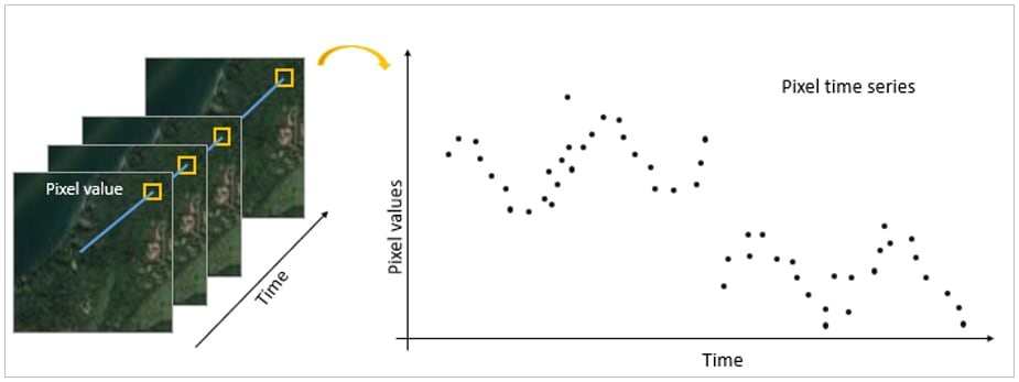
Time series analysis in satellite-based ML applications requires careful attention to the temporal resolution of both your labels and imagery. In the context of MOSAIKS, you may opt for different strategies depending on the frequency of satellite acquisitions and how quickly your outcome of interest changes.
18.1.1 Temporal alignment
When aligning data in time, consider:
Label frequency: How often are ground measurements collected? For instance, annual crop yields, monthly economic indicators, or even daily weather observations. The granularity of these data points will guide how to match them to your satellite-derived features.
Imagery availability: How frequently can you obtain clear satellite images of your area of interest? High revisit rates enable more frequent observations, but factors like cloud cover or sensor anomalies may reduce the actual number of usable images.
Change detection: How quickly does your variable of interest change? Urban development may unfold over months or years, whereas flood events can occur within days. Matching the temporal granularity of your features to the dynamics of your phenomenon is crucial.
18.1.2 Seasonal patterns
Both natural and human-driven processes often exhibit strong seasonal signals:
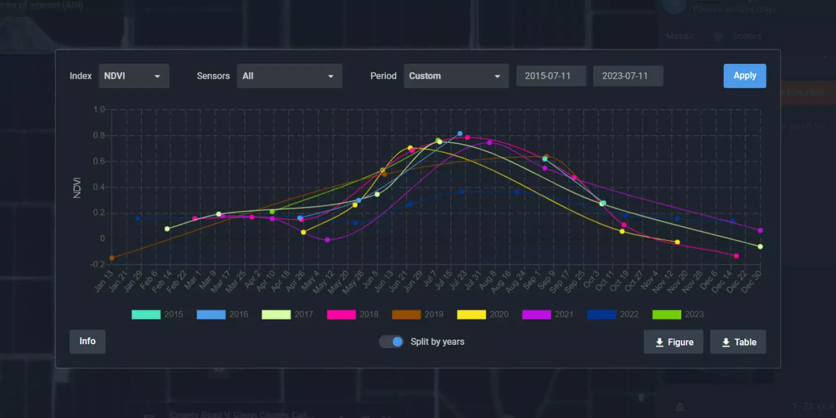
Natural cycles: Vegetation growth, snow cover, and water extent are all influenced by seasons. For example, NDVI metrics might be more informative during peak growing seasons (Figure 18.2).
Human activities: Cropping cycles, holiday travel, and heating or cooling demand are just a few examples of how human behavior can vary throughout the year. These temporal rhythms can introduce systematic patterns in your data.
Feature extraction: Because satellite observations reflect surface conditions, different times of the year may require distinct feature sets. For example, reflectance values change when vegetation is senescent vs. when it is fully grown. Similarly, atmospheric conditions (like haze) may be more prevalent in certain seasons.
18.1.3 Challenges in time series applications
Although the potential benefits of time series analysis are significant, there are a few common pitfalls:
18.1.3.1 Data gaps
Cloud cover: In regions with high cloud coverage, usable imagery can be sparse, leading to irregular time intervals between valid observations.
Satellite maintenance or sensor dropout: Even short interruptions in satellite operations can reduce data availability.
Orbital patterns: Some satellites have specific revisit schedules, meaning certain areas might not be imaged as frequently as others, leading to patchy time series data.

For more information on cloud cover and its impact on satellite data, see Flores-Anderson et al. 2023.
18.1.4 Pre-processed satellite products
Several satellite providers offer pre-processed data products specifically designed for time series analysis. These products handle common challenges like cloud cover and normalization:
18.1.4.1 MODIS vegetation indices
- 16-day or monthly composites of vegetation indices (e.g., NDVI, EVI)
- Automated cloud masking and quality control
- Surface reflectance values normalized for atmospheric effects
- Global coverage at 250m-1km resolution since 2000
- Ideal for monitoring seasonal vegetation dynamics
18.1.4.2 Planet Basemap
- Quarterly visual composites from multiple PlanetScope satellites
- Cloud-free mosaics using best available pixels
- Color-balanced and radiometrically calibrated
- Global coverage at ~4.7m resolution
- Suitable for tracking gradual land use changes
18.1.4.3 Harmonized Landsat-Sentinel (HLS)
- Combined product using Landsat 8-9 and Sentinel-2 imagery
- 2-3 day revisit frequency at 30m resolution
- Atmospherically corrected and co-registered
- Consistent surface reflectance values between sensors
- Enables dense time series from 2013-present
These products reduce the preprocessing burden for users but may not capture rapid changes that occur between compositing periods. The choice between using raw imagery or pre-processed products depends on the temporal resolution needed for your specific application. These data products and how to use them will be covered in greater detail in Chapter 9 and Chapter 10.
18.1.4.4 Temporal consistency
Sensor drift: Over time, satellite sensors can degrade or drift, influencing the consistency of your data. Proper calibration can mitigate these issues.
Multi-sensor calibration: If you are combining data from multiple satellites in a constellation, ensure that differences in sensor sensitivity or bands do not introduce spurious signals in your time series.
18.1.4.5 Storage and computation
Data volume: Each additional time step in your analysis increases the storage and processing requirements.
Temporal correlation: Many time series phenomena exhibit autocorrelation, which can influence how you design and train models. Standard ML algorithms assume independence between samples, so specialized methods or features (such as lagged features) may be required to handle temporal dependencies.
18.2 Approaches to time series modeling
Below are three common strategies for incorporating time series data within a MOSAIKS-like framework. Each approach has trade-offs in terms of complexity, computational cost, and interpretability.
18.2.1 Feature stacking
In a feature-stacking approach, you generate MOSAIKS features for multiple time steps and then concatenate them into a single feature vector. This is straightforward but can lead to very large feature spaces if you have many time points.
Compute features for each time period: Run your MOSAIKS feature extraction for each quarter, month, or year—whatever time granularity is relevant.
Concatenate features: Combine them into a single vector, ensuring that naming conventions keep time steps distinguishable.
Model training: Input the stacked features into your preferred machine learning algorithm (e.g., linear regression, random forest, or neural network).
Example (quarterly stacking):
# Create feature names for each quarter
features_Q1 = [f'X_{i}_Q1' for i in range(1000)]  # X_0_Q1, X_1_Q1, ..., X_999_Q1
features_Q2 = [f'X_{i}_Q2' for i in range(1000)]  # X_0_Q2, X_1_Q2, ..., X_999_Q2
features_Q3 = [f'X_{i}_Q3' for i in range(1000)]  # X_0_Q3, X_1_Q3, ..., X_999_Q3
features_Q4 = [f'X_{i}_Q4' for i in range(1000)]  # X_0_Q4, X_1_Q4, ..., X_999_Q4

# Combine features names for all quarters
features_annual = features_Q1 + features_Q2 + features_Q3 + features_Q4

# Total length = 4,000 features for four quarters
features_df = pd.DataFrame(data=features, columns=features_annual)
This approach is typically suitable for annual or seasonal data where the number of time steps remains manageable. However, it may be less practical if you have daily or weekly observations over several years.
18.2.2 Temporal aggregation
In temporal aggregation, you compute features at a higher frequency but then summarize them over a time window:
Extract features at a high frequency: This provides a rich temporal view.
Aggregate: Compute statistical summaries such as the mean, max, or variance of each feature across the chosen time window. Common windows include daily, weekly, monthly, and quarterly aggregations.
Model with aggregated features: The aggregated features can represent dynamic processes while controlling the dimensionality of your dataset.
This method captures general trends and reduces noise from cloud cover or other transient factors. However, important temporal nuances (like specific short-lived events) might be lost in the aggregation.
18.3 Demeaning
Evaluation over time
18.3.1 Sequential modeling
For phenomena where temporal order is crucial and frequent observations exist, sequential modeling can be more powerful:
Feature extraction: Maintain the time dimension in your feature matrix (e.g., one matrix per location, with time as rows and features as columns).
Apply time series modeling: Techniques like LSTM (Long Short-Term Memory) networks, temporal convolutional networks, or classical state-space models (e.g., ARIMA) can handle temporal dependencies explicitly.
Lagged relationships: Incorporate features from previous time steps to capture delayed effects (e.g., precipitation from last month affecting vegetation today).
Although these methods provide a more nuanced view of temporal processes, they require additional modeling expertise and computational resources.
Start with a simpler approach like feature stacking or temporal aggregation. If you find that your phenomenon has rapid or complex temporal dynamics that aren’t well-captured by these methods, then explore more advanced sequential models.
18.4 Hands on with time series data
In lieu of time series MOSAIKS features, we will instead demonstrate similar examples using MODIS NDVI data. This will allow us to explore the challenges and opportunities of time series analysis without the need for custom feature extraction.
NOTE: UPDATE ME with new notebook link.
↓↓↓↓↓↓↓↓↓↓↓![]()
Remember to click File -> Save a copy in Drive to save any changes you make.
18.5 Filling temporal gaps
When working with time series data, you may encounter missing values due to cloud cover, sensor issues, or other factors. Here are some common strategies for filling these gaps:
18.6 Summary
Handling time series in satellite-based ML workflows requires balancing data volume, temporal alignment, and modeling complexity. While feature stacking can be effective for low-frequency or seasonal processes, more sophisticated techniques may be needed to capture high-frequency changes or long-range temporal dependencies. Ultimately, the “best” approach depends on the nature of your target variable, data availability, and the resources at your disposal.
In the next chapter we will look at