7  Preparing labels

This chapter is under review and may need revisions.

7.1 Overview

In this chapter, we discuss the process of preparing labels for use with MOSAIKS features. Labels are the observed values we aim to predict with our model—such as crop yields, forest cover, or any variable of interest. They can come in many spatial formats (e.g., points, polygons, or gridded rasters), but they must include a spatial component. We use this spatial information to join the labels with MOSAIKS features, which are also spatially explicit.

Although MOSAIKS offers many optional steps, two components are essential:

1. Ground observations (labels)
   
2. Satellite features

Both datasets must align in spatial resolution and contain appropriate geographic data for merging.

7.2 MOSAIKS Grid

Before we talk about labels, we must first understand the resolution that the MOSAIKS features are offered in. The resolution you choose will serve as the target resolution for your summarizing your labels.

7.2.1 Resolution

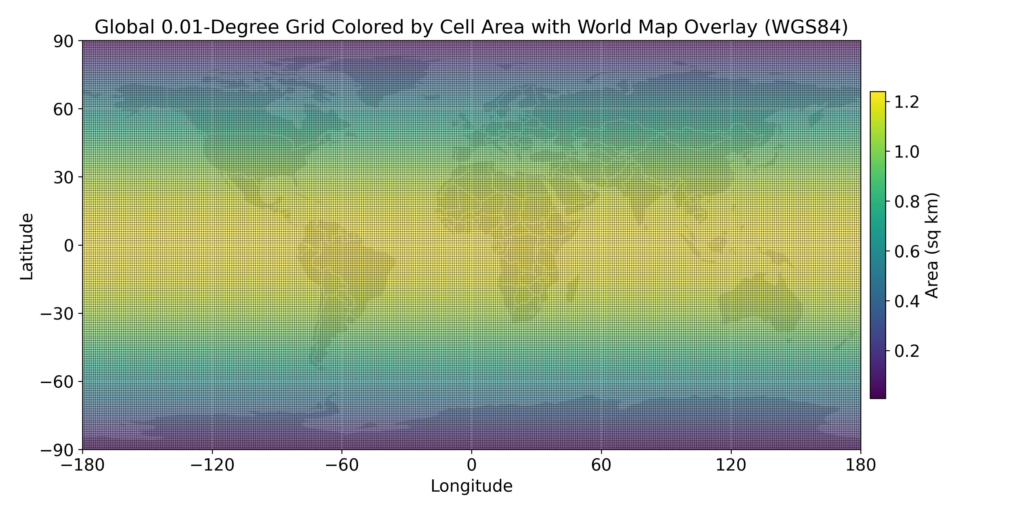
The standard resolution of MOSAIKS is a global grid at 0.01° resolution. Each grid cell is approximately 1 km² at the equator. The grid is often represented as a point grid, where each point is the center of a grid cell. This means that standard MOSAIKS features come with a latitude and longitude coordinate, which is the center of the grid cell.

MOSAIKS grid cell centroids are rounded to 0.005 degrees and are spaced by 0.01 degree (e.g., 10.005, 10.015, 10.025,…).

Figure 7.1: Visual representation of a standardized grids at varying resolutions (δ) with the highest resolution on the left, and lower resolutions moving right. Source: Rolf et al. 2021 Figure 3 c.

7.2.2 Advantages of the MOSAIKS grid

The MOSAIKS grid has several advantages. The primary advantage is that it helps avoid overlapping labels. Often label data come with coordinates which are unevenly spaced. If you are forced to align your labels to a grid and summarize within cells, you can avoid bleed over from one label to another. This is especially important when you are working with data that has a high degree of spatial autocorrelation.

The MOSAIKS API is designed to predict outcomes at scales of 1 km² or larger. Custom solutions are possible for higher-resolution applications (see Chapter 14).

7.2.3 Disadvantages of the MOSAIKS grid

The MOSAIKS grid is defined in degrees, therefore the area of a given cell varies with latitude. Near the equator, each cell is approximately 1 km², while at higher latitudes the area decreases as the distance between meridians (longitude lines) converges.

Figure 7.2: The area of a grid cell at different latitudes.

7.2.4 Choosing your resolution

We know from Chapter 3 that the MOSAIKS API offers features at 0.01°, 0.1°, 1°, ADM2, ADM1, and ADM0 resolutions. In all cases, features are computed at 0.01° resolution and then aggregated to the desired resolution. If you plan on using the API to download features, you need to make sure your labels are at the same resolution as the features you plan to download.

7.3 Ground Observations

7.3.1 Resolution

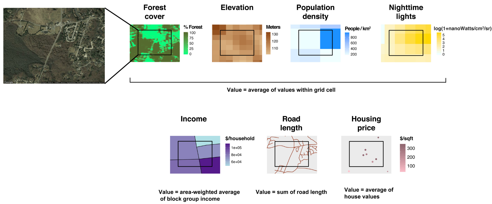
Preparing label data for MOSAIKS depends on location, extent, time, and resolution. When observations have a resolution finer than 1 km², you must select or aggregate them to match the features you plan to use. MOSAIKS can incorporate labels from raster, point, polygon, or vector data. In Chapter 8, we will demonstrate how to prepare labels for each input type.

Figure 7.3: Examples of label data formats that can be easily integrated into the MOSAIKS pipeline. Label data of any spatial format that can be aggregated to at least the scale of 1km² (or larger) can be used directly in combination with MOSAIKS imagery features for downstream prediction tasks. Examples shown here are from Rolf et al. (2021) and include: forest cover, elevation, population, and nighttime lights datasets (all raster format); income data (polygon format); road length (vector format); and housing price data (point format). Source: Rolf et al. 2021 Supplementary Figure 4.

7.3.2 Administrative level data

In some cases, you will find labels for administrative regions (states, districts, etc.). In this case, it might not come with any geographic information other than a place name. You can usually find the relevant geographic information online. A good resource for this is the Global Administrative Areas (GADM) database, which provides the boundaries for administrative division at various levels for completely free.

Figure 7.4: Global Human Development Index (HDI) data at the first sub-national level of administrative division (ADM1). Source: Smits & Permanyer 2019.

7.3.3 Challenges of administrative data

Data can be messy. There are two main challenges with administrative data.

1. Name matching: The names in your dataset might not match perfectly with the names in the GADM database or in the MOSAIKS API. Finding a way to comprehensively match these can be time consuming and difficult.

2. Boundary changes: Administrative boundaries are not always static. Some regions undergo frequent changes and you need to ensure your data matches the boundaries of the features you use.

7.3.4 Sample Size

Increasing sample size (N) often yields higher model performance. MOSAIKS has demonstrated effectiveness across a wide range of sample N. The sample size depends on the spatial (and potentially temporal) resolution of your label data. For instance, if each record is aggregated at the county level, then N equals the number of counties. Incorporating multiple time periods can increase N but also requires more imagery to be featurized (see Chapter 14).

As a general rule, a minimum of 300 observations for model training is recommended, though every application is unique and may require more or fewer observations.

The original MOSAIKS publication (Rolf et al., 2021) evaluated models with sample sizes from 60,000 to 100,000. In most cases there were only modest performance declines with a few hundred observations (Figure 7.5). In recent crop yield experiments, high performance (R² = 0.80) was achieved with around 400 observations, provided the data were cleaned and aggregated to a district level. It is important to note that the original crop yield dataset included interview records from thousands of farmers across the study country. While this data has a large sample size, it is messy. In this case, a clean dataset with a low number of observations was preferred to a large but noisy dataset.

Figure 7.5: Model performance for all seven tasks while varying the number of random convolutional features K and holding N = 64,000 (left) and while varying N and holding K = 8,192 (right). Shaded bands indicate the range of predictive skill across five folds. Lines indicate average accuracy across validation folds. Source: Rolf et al. 2021 Figure 3 b.

7.3.5 Data Types

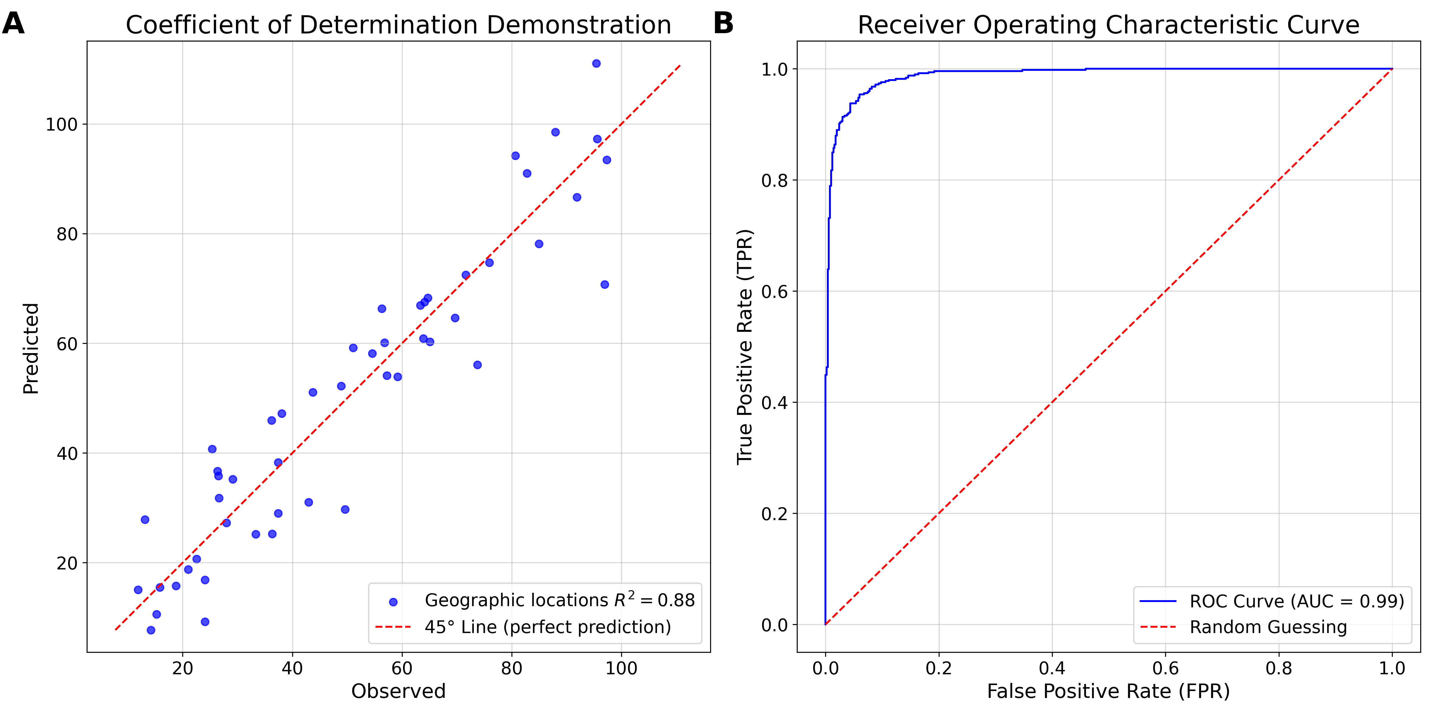
MOSAIKS can accommodate both continuous labels (e.g., fraction of area forested) and discrete labels (e.g., presence/absence of mine). Data type informs model development, performance evaluation, and choice of metric (see Chapter 16). Continuous variables often use coefficient of determination (R²), while discrete variables often use Receiver Operating Characteristic Area Under the Curve (ROC AUC).

Figure 7.6: A The coefficient of determination (R²) is a measure of how well the model fits the data. It ranges from 0 to 1, where 1 indicates a perfect fit. The closer each point is to the 45 degree line, the higher the better the model fit and the higher the score will be. B The Receiver Operating Characteristic (ROC) curve is a graphical representation of the true positive rate (sensitivity) against the false positive rate (1-specificity). The area under the curve (AUC) ranges from 0 to 1, where 1 indicates a perfect model. Diagonal line is equivalent to random guessing.

The data type may also effect how the data is cleaned and prepared. For example you may have a dataset of mining locations across a country. If you are interested in predicting the presence of mining, you may want to convert this to a binary variable where a 0 indicates no mining and a 1 indicates mining. Alternatively, you may be interested in predicting the area of mining in each location, in which case you might need to calculate the area of the mining polygons to make the variable continuous.

7.4 Joining Data

7.4.1 Merging Labels with MOSAIKS Features

To merge labels with features, you must align the geographic location of both datasets. The native resolution MOSAIKS feature files have rows for each location and columns with longitude, latitude, and features. Your label dataset must also have columns for longitude, latitude, and label values (at minimum). Alternatively, aggregated features will come with the name of the administrative region (e.g., district) and the features. You can join this with your label data by matching the district names.

7.4.2 Example Data Structure

A simple example: district-level crop yield labels might look like:

Observation	District	Year	Crop Yield
1	Chibombo	2019	1.520
2	Kabwe	2019	1.878
…	…	…	…
N	Kitwe	2019	2.383

Table 7.1: Fictional crop yield data for districts in Zambia.

MOSAIKS features at this same resolution might look like:

Observation	District	Year	Feature 1	Feature 2	…	Feature K
1	Chibombo	2019	4.2	11.6	…	12.7
2	Kabwe	2019	2.9	5.3	…	11.2
…	…	…	…	…	…	…
N	Kitwe	2019	10.6	1.1	…	2.2

Table 7.2: Fictional MOSAIKS feature data for the same districts.

After a spatial join, you end up with a merged dataset:

Observation	District	Year	Crop Yield	Feature 1	Feature 2	…	Feature K
1	Chibombo	2019	1.520	4.2	11.6	…	12.7
2	Kabwe	2019	1.878	2.9	5.3	…	11.2
…	…	…	…	…	…	…	…
N	Kitwe	2019	2.383	10.6	1.1	…	2.2

Table 7.3: Example of joined data with both labels and features.

In the above example, our geographic location is the district and our label is the crop yield (mt/ha). We then have K columns containing the features and N observations.

7.5 Data Cleaning Considerations

7.5.1 Coordinate Reference Systems (CRS)

The default coordinate reference system used by MOSAIKS is World Geodetic System 84 (WGS 84). The standardized code that defines WGS 84 is “EPSG:4326”. EPSG stands for the European Petroleum Survey Group, which maintains a database of coordinate systems and projections. The WGS 84 coordinate system is the most commonly used coordinate system for GPS data.

Figure 7.7: Nine small-scale map projections.

If your data is not in WGS 84, you will need to reproject it to this coordinate system before joining it with MOSAIKS features.

7.5.2 Label Quality

Confirm that label values are within expected ranges, deal with any outliers or missing data, and ensure units are consistent and numeric fields are properly formatted. This book does not go into a great deal of detail on cleaning messy data. This topic is covered in exhaustive detail in the book R for Data Science.

7.5.3 Temporal Alignment

If you have time series labels, you will need to compute custom features for each time period. See Chapter 14 for more information on how to do this and ?sec-model-temporal for guidance on modeling time series data with MOSAIKS features.

7.5.4 Data Formats

MOSAIKS can work with several common spatial data formats:

Data Type	Common File Formats	Description	Example	Geographic information
Point Data	CSV, GeoJSON, Shapefile	Coordinate pairs	Places of interest	geometry
Line Data	GeoJSON, Shapefile	Geographic lines	Roads, rivers	geometry
Polygon	GeoJSON, Shapefile	Geographic areas	Buildings, fields	geometry
Raster	GeoTIFF, NetCDF	Gridded data	Forest cover, elevation	grid
Administrative	CSV	Administrative boundaries	Districts, states	place names

Table 7.4: Common spatial data formats with file types, descriptions, examples, and indication of how the spatial information is stored.

When working with large datasets, converting to efficient data formats such as Parquet, Feather, GeoTIFF, or Zarr can reduce memory usage and improve processing speed.

7.6 Summary

The most important considerations when preparing labels for MOSAIKS are spatial resolution, sample size, data type, and data quality. Once you have prepared your labels, you can join them with MOSAIKS features to create a dataset ready for modeling.

A demonstration of how to process data for the data types in Table 7.4 is provided in the next chapter. This notebook will cover the process of creating a MOSAIKS grid, downloading data, and creating a label dataset at the grid level (0.01 degree) and at the second level of administrative division (ADM2).

7.6.1 Labels data checklist

For optimal use with MOSAIKS, label data should be:

• Consistently geolocated as point, polygon, vector, or raster data
• Aggregable to ≥ 1km² resolution
• Observable in daytime satellite imagery (directly or indirectly)
• Recent or slow-changing if using current API features
• Sample size N≥300 (larger samples generally perform better)
• Cleaned and formatted for modeling

Looking forward

In the next chapter, we’ll look at practical guidance for preparing label data for use with MOSAIKS including data cleaning and aggregation.