9 Choosing imagery
This chapter is under review and may need revisions.
9.1 Background
The number of Earth observation satellites has grown exponentially in recent years, driven by advancements in technology, reduced launch costs, and an increasing demand for environmental, economic, and societal insights.
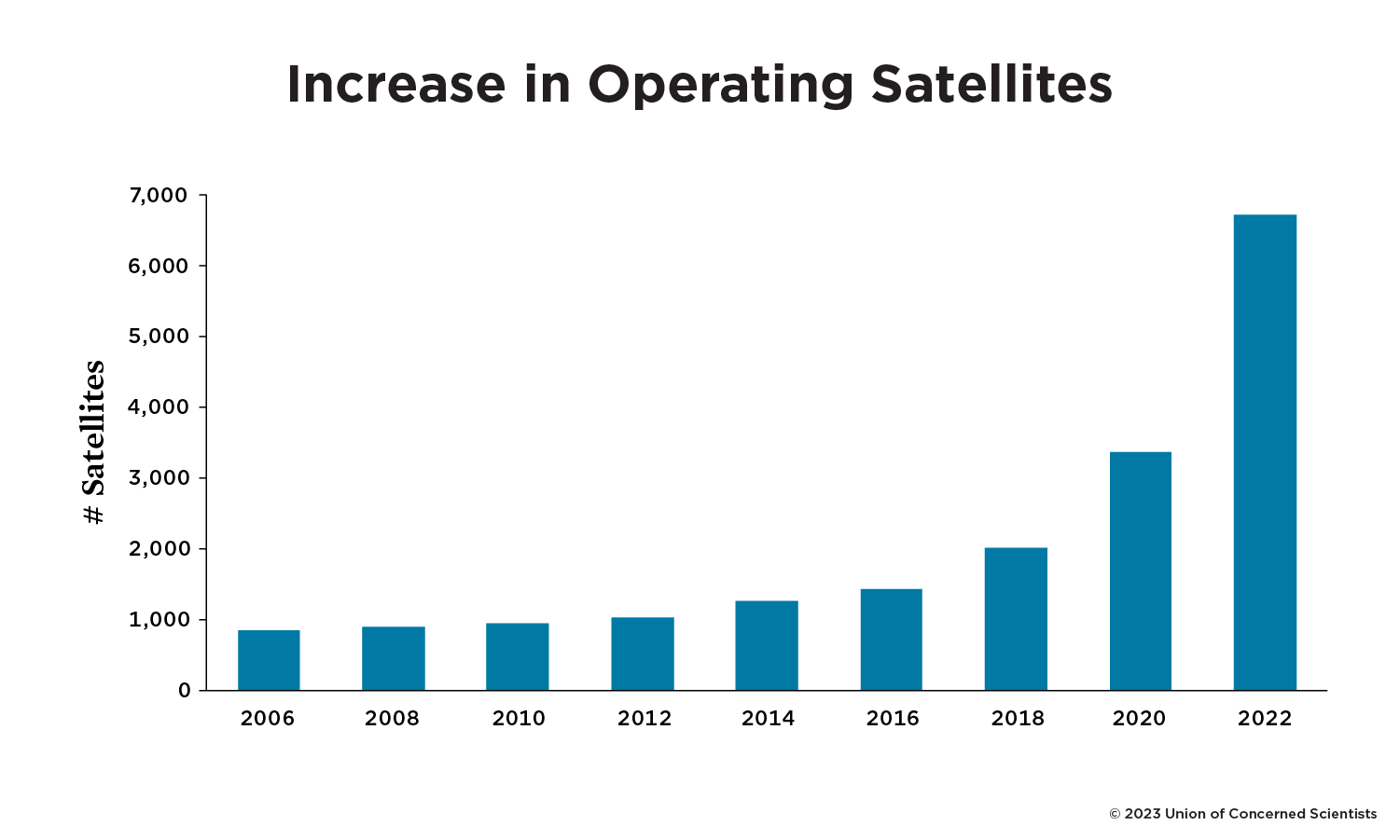
Alongside this growth, the quality of satellite imagery has improved significantly, with higher spatial, temporal, and spectral resolutions becoming the norm. The proliferation of satellites, coupled with enhanced imaging capabilities, has resulted in an unprecedented volume of data, offering researchers and practitioners a wealth of opportunities—but also presenting challenges in navigating the diversity of data products and selecting those most suited to specific applications.

MOSAIKS leverages satellite imagery to generate high-quality training data for machine learning models. In this chapter, we explore the key factors to consider when choosing satellite imagery for use with MOSAIKS, including spatial and spectral resolution, temporal frequency, cloud cover, and processing levels.
Access the UCS Satellite Database for a comprehensive list of Earth observation satellites, including key specifications and operational details.
9.2 Overview
When selecting satellite imagery for use with MOSAIKS, several key factors need to be considered. The choice of imagery should be guided by your specific research needs, label characteristics, and practical constraints like cost and processing requirements. Different use cases, such as monitoring vegetation, mapping urban areas, or tracking climatic variables, may require specific imaging capabilities, making it essential to align satellite features with your intended application. Additionally, trade-offs between resolution, temporal frequency, and accessibility can significantly influence the feasibility of your analysis.
For example, high-resolution data from commercial satellites might offer detailed insights but could be prohibitively expensive for large-scale applications. On the other hand, publicly available datasets like Sentinel-2 provide cost-effective options, albeit with potentially coarser resolutions or limited spectral coverage. Understanding these trade-offs is essential to ensure the optimal use of resources.
| Consideration | Description |
|---|---|
| Availability | The availability and cost of imagery from public and private sources. |
| Time range | The time period for which satellite images are available. |
| Temporal resolution | The frequency at which satellite images are captured (e.g., daily, weekly). |
| Spatial resolution | The spatial resolution of the satellite sensor (e.g., 10m, 30m, 250m). |
| Spectral resolution | The specific wavelengths captured by the sensor (e.g., RGB, NIR, SWIR). |
| Sensor type | The type of sensor used (e.g., optical, radar, thermal). |
| Cloud cover | Cloud cover or other atmospheric interference. |
| Processing level | The preprocessing applied (e.g., orthorectification, normalization). |
9.3 Availability
9.3.1 Public Satellites
Public satellite programs offer free or low-cost imagery with global coverage. These programs, funded by government agencies, provide extensive data for scientific research and environmental monitoring. They are particularly valuable for long-term studies, thanks to consistent data archives spanning decades, and for projects with limited budgets. Publicly funded satellites often balance moderate resolutions with frequent revisit times, ensuring data accessibility and temporal consistency.
| Satellite | Sensor Type | Resolution | Revisit Time | Special Features |
|---|---|---|---|---|
| Sentinel-2 | Optical | 10-60m | 5 days | 13 spectral bands |
| Landsat 8/9 | Optical | 15-100m | 16 days | 11 spectral bands |
| MODIS | Optical | 250m-1km | Daily | 36 spectral bands |
| Sentinel-1 | Radar (C-band) | 5-40m | 6-12 days | Synthetic Aperture Radar (SAR) |
| NISAR | Radar (L- and S-band) | TBD | Launching 2024 | Dual-band SAR |
| VIIRS | Other | 375m-750m | Daily | Daily global coverage |
| ASTER | Other | 15-90m | 16 days | 14 spectral bands |
| NICFI | Optical | 4.77 m | monthly composite | Tropical forest monitoring |
9.3.2 Private Satellites
Private satellite programs often provide higher resolution imagery, greater specialization, and more frequent revisits than public programs, but typically at a higher cost. These satellites are particularly useful for applications requiring fine detail, such as urban mapping, infrastructure monitoring, or precision agriculture. Private providers often offer custom data products, tailored delivery timelines, and advanced analytics, which can be invaluable for time-sensitive or commercially driven projects. However, the higher costs associated with private imagery may limit their use for large-scale or long-term studies without significant funding.
| Satellite | Sensor Type | Resolution | Revisit Time | Special Features |
|---|---|---|---|---|
| Maxar WorldView | Optical | 31cm (panchromatic), 1.24m (multispectral) | Varies | Very high resolution |
| Planet SkySat | Optical | 50cm (panchromatic), 1m (multispectral) | Varies | Compact, agile satellites |
| Airbus Pleiades | Optical | 50cm (panchromatic), 2m (multispectral) | Varies | Very high resolution |
| Planet PlanetScope | Optical | 3-5m | Daily | Large constellation |
| Planet RapidEye | Optical | 5m | 5.5 days | Designed for agriculture |
| SPOT | Optical | 1.5-6m | 26 days | Long-standing program |
| ICEYE | Radar (X-band) | <1m | Frequent | High revisit SAR |
| Capella Space | Radar (X-band) | 50cm | Frequent | High resolution SAR |
| GHGSat | Specialized | TBD | Varies | Greenhouse gas monitoring |
9.3.3 Cost considerations
Remember that the most expensive or highest resolution imagery isn’t always the best choice. Balancing your needs with practical constraints—like budget, storage capacity, and processing expertise—can often yield better long-term outcomes than simply opting for the highest-specification option.
Selecting satellite imagery involves not only the direct expense of acquiring data but also a range of indirect or “hidden” costs. When factoring these into your overall budget, consider how frequently you need updates, the extent of pre- or post-processing required, and whether your team has the technical skills to work with complex datasets. Some satellites and data portals also bundle analytics and cloud storage into subscription services, which can alleviate infrastructure demands at an additional cost.
Below is an example of how imagery costs might break down, offering a quick reference for typical price points and considerations across different data sources:
| Cost Tier | Approximate Range | Example Missions/Programs | Key Considerations |
|---|---|---|---|
| Free Public Data | $0 | Landsat (30m), Sentinel (10m), MODIS (250m–1km), VIIRS (375m–750m) | Government-funded; widely used for large-scale or long-term projects; moderate resolution. |
| Medium-Resolution | $1–5 per km² | SPOT (1.5–6m) | Relatively affordable for moderate detail; suitable for regional analyses. |
| High-Resolution | $5–15 per km² | Planet (3–5m), RapidEye (5m) | Useful for more detailed studies; frequent revisit can drive up cost if coverage is large. |
| Very High Resolution | $15–25 per km² | WorldView (sub-meter), SkySat (0.5–1m) | Offers fine-grained detail but at a premium; cost can escalate quickly for large areas. |
| Subscription Services | Variable | Some commercial data providers bundle storage & analytics | Often convenient “one-stop shop,” but pricing may be unpredictable or scale poorly. |
In addition to these basic acquisition costs, you should also consider:
-
Data Storage and Computing: Large volumes of high-resolution imagery require greater storage space and more computational power for processing.
-
Expertise and Training: Interpreting complex datasets (such as radar or hyperspectral imagery) often demands specialized skills.
-
Software Licenses: Proprietary GIS or image processing software can add to your operational budget.
- Cloud Infrastructure: Commercial cloud solutions can handle large-scale processing but may entail ongoing subscription fees.
Carefully weighing these direct and indirect expenses will help you choose imagery that optimizes both scientific value and cost-effectiveness.
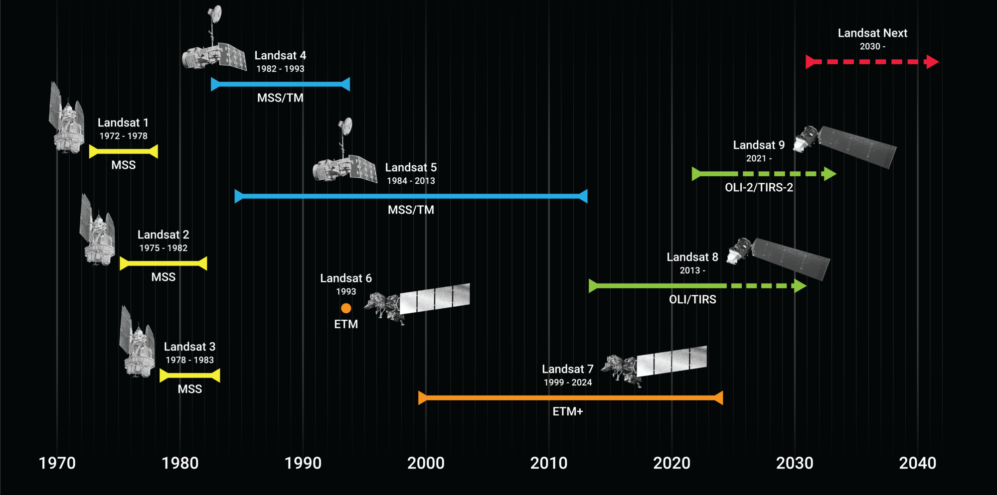
9.4 Time range
The operational lifespan and launch history of a satellite mission are essential considerations when selecting imagery for your project. Older programs such as Landsat offer data archives spanning several decades, making them valuable for long-term change detection or historical analyses. In contrast, newer satellites like Sentinel, launched in 2014, provide data with more advanced sensor technologies but cover a shorter temporal window.
When deciding on a time range, it is important to assess the historical depth your study demands, as well as the consistency of sensor technology over that period. Projects that require comparisons across many years benefit from missions with well-documented calibration procedures and stable sensor performance over time. You may also need to factor in whether future data continuity is guaranteed by planned satellite launches or extended operational budgets. For instance, Landsat’s multi-generational program ensures a relatively consistent data record, while newer constellations might offer superior capabilities but face funding uncertainties that could impact long-term availability.
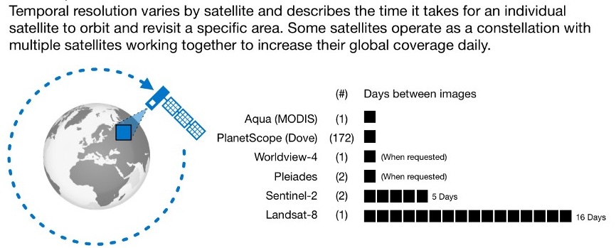
9.5 Temporal resolution
Temporal resolution, or revisit frequency, dictates how often a satellite images the same location. Higher revisit rates allow you to monitor rapidly changing phenomena, such as vegetation growth cycles or flood dynamics, and respond more quickly to evolving events. However, satellites that pass over more frequently often trade off spatial or spectral detail.
When selecting temporal resolution, consider the pace at which your target variables change. Monitoring daily fluctuations in crop conditions requires denser time series than an annual assessment of deforestation. Cloud conditions in your study area can also influence the effective revisit rate: if clouds frequently obscure the land surface, you may need a satellite constellation with multiple imaging opportunities or a sensor that can “see” through clouds, like radar (SAR). Budget and data processing capacities further shape your decision, since frequent imaging can lead to increased data storage needs and processing overhead.
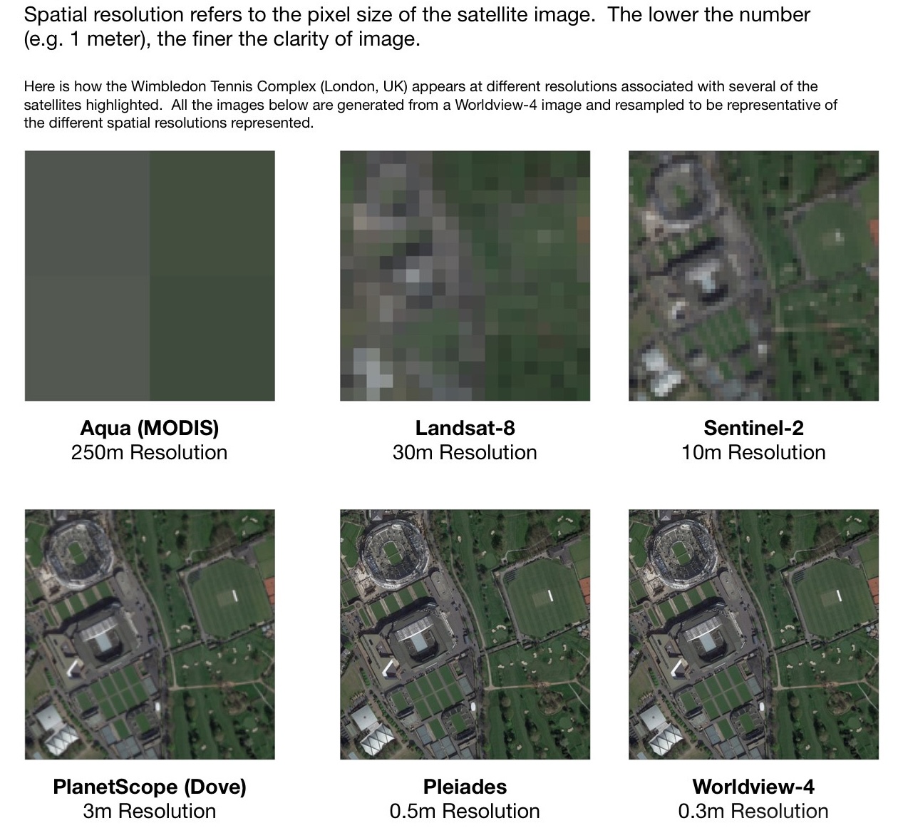
9.6 Spatial resolution
Spatial resolution of the satellite sensor determines the level of detail captured in satellite imagery. At higher resolutions, features such as individual trees, vehicles, or small buildings are discernible. Lower resolutions provide broader overviews of landscapes—suitable for regional-scale studies like climate analysis or large-area land cover mapping—but may miss fine-grained changes in smaller features.
Although very high resolution imagery (below one meter) can yield rich information, it often carries higher costs and storage requirements. Meanwhile, moderate resolutions (10–30 m) balance meaningful detail with affordability and manageable data volumes. Your choice should account for the physical size of the features relevant to your labels, the scale of your study area, and the computational resources at your disposal. In many cases, public missions like Sentinel-2 or Landsat offer practical resolutions (10–30 m) that suffice for broad-scale analyses without incurring the expense associated with commercial high-resolution imagery.
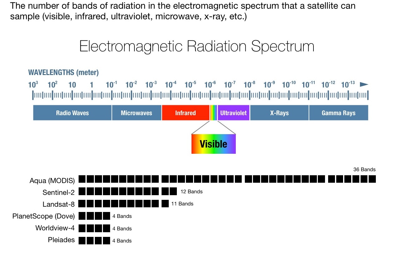
9.7 Spectral resolution
Spectral resolution refers to the sensor’s ability to measure discrete wavelengths across the electromagnetic spectrum. Different materials—such as vegetation, water, and urban infrastructure—exhibit distinct spectral signatures, so capturing multiple bands can enhance classification accuracy and thematic mapping. For instance, near-infrared (NIR) bands are extremely valuable for quantifying vegetation health, while shortwave infrared (SWIR) can help distinguish between minerals and moisture content.
Choosing an appropriate spectral resolution involves balancing the number and width of bands with the specific thematic information you need. Sensors that capture only visible light (RGB) may suffice for broad land cover discrimination, whereas applications such as agricultural health monitoring often benefit from additional NIR or SWIR coverage. Thermal or microwave bands can also be critical in specialized domains—like thermal anomaly detection or soil moisture estimation—and thus influence the utility of certain satellite platforms for specific scientific or operational goals.
9.8 Sensor type
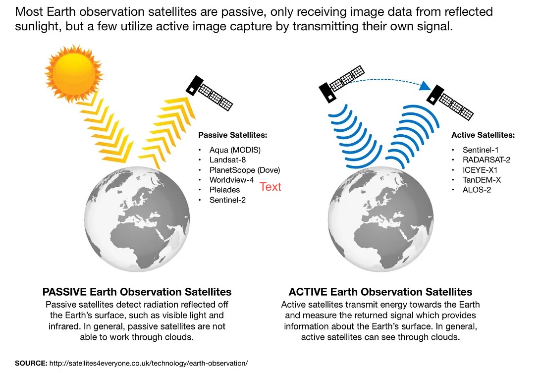
Satellite sensors can generally be characterized as passive or active instruments. Both categories have distinct advantages and limitations that influence their suitability for particular applications.
Passive sensors measure natural radiation, typically reflected sunlight (optical) or emitted heat (thermal). Because they rely on external energy sources, data collection can be constrained by sunlight availability and atmospheric conditions. However, optical imagery from passive sensors often offers intuitive color representations, making it easier to interpret. Thermal bands can reveal heat signatures useful in land surface temperature studies.
Active sensors emit their own energy and record the backscatter signal. Radar systems (e.g., SAR) and LiDAR instruments fall under this category. They can penetrate clouds, operate at night, and measure surface characteristics such as roughness or elevation. On the downside, the data are often more complex to process and interpret, requiring specialized expertise and software.
Below is a simple comparison of these sensor types:
| Sensor Type | Examples | Operating Principle | Pros | Cons |
|---|---|---|---|---|
| Passive | Optical, Thermal | Measures naturally available reflected energy (sunlight or emitted heat) | Easier to interpret; often intuitive (e.g., RGB images) | Limited by cloud cover and sensitive to atmospheric conditions |
| Active | Radar (SAR), LiDAR | Emits energy and measures return signals | Can penetrate clouds, capture data day or night | Data may require more complex processing |
Understanding which sensor type best aligns with your research needs is crucial. For instance, if your study area is frequently cloudy, a radar-based approach can offer more reliable coverage. Alternatively, optical sensors might be sufficient for regions with seasonal cloud-free windows or for general land-cover classification when consistent sunlight is available.
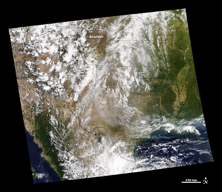
9.9 Cloud cover
Cloud cover is one of the most persistent challenges in working with optical satellite imagery, as clouds and shadows can degrade the quality of the collected data. In regions with frequent cloudiness, images may require additional processing or longer acquisition windows to achieve acceptable coverage. Strategies to address this issue include applying cloud masking algorithms, merging multiple images to create a cloud-free composite, or using radar-based satellites that penetrate clouds.
Optical sensors, such as those on Sentinel-2 or Landsat, often include quality assurance layers that flag pixels contaminated by clouds. Filtering out these pixels improves data reliability but reduces the amount of usable imagery, potentially limiting temporal coverage in cloudy regions. On the other hand, radar missions like Sentinel-1 or ICEYE remain largely unaffected by cloud conditions, offering consistent coverage at the cost of different data characteristics and additional expertise required for radar data interpretation. Weighing these trade-offs helps in choosing imagery that meets both your accuracy requirements and your practical constraints.
9.10 Processing levels
Satellite data are distributed at various processing levels, ranging from unprocessed instrument measurements to derived products that are nearly ready for analysis. Selecting a processing level that aligns with your project’s technical requirements can streamline workflows and ensure consistent results.
Below is a general outline of commonly encountered processing levels:
| Level | Description | Typical Use Case |
|---|---|---|
| Level 0 | Raw instrument data with minimal or no preprocessing. Often not orthorectified or radiometrically calibrated. | Rarely used for general analysis due to complexity. |
| Level 1 | Radiometric calibration and basic geometric corrections. Sometimes subdivided (e.g., 1A, 1B, 1C). | Suitable if you need control over final atmospheric corrections or custom workflows. |
| Level 2 | Surface reflectance products with atmospheric corrections applied, often including cloud/shadow masks. | Most common for analyses requiring accurate reflectance values and multi-temporal comparisons. |
| Level 3 | Derived or composite products (e.g., mosaics, NDVI layers, gap-filled data). | Ideal for thematic applications that benefit from aggregated or pre-processed data. |
Additional processes often applied during or after these levels include:
- Orthorectification: Removal of geometric distortions caused by sensor tilt, terrain relief, and Earth curvature. Ensures accurate spatial representation for mapping and analysis.
- Atmospheric correction: Adjustment for atmospheric effects (aerosols, water vapor) to standardize reflectance values across different times or sensors.
- Radiometric calibration: Conversion of raw sensor counts to physical units like reflectance or brightness temperature, enabling consistent comparisons among images from different sensors and acquisition dates.
Knowing which processing steps your data provider already performs helps you avoid redundant work and ensures you acquire data that meet your accuracy requirements. For instance, if you need consistent multi-temporal comparisons, opt for Level 2 or higher to minimize atmospheric variations. Conversely, if you prefer to perform your own corrections and calibrations, Level 1 might offer greater flexibility at the cost of added complexity.
9.11 Choosing the right combination
Selecting the right combination of spatial, spectral, temporal, and sensor characteristics can feel overwhelming, given the numerous satellites and data products available. This choice often comes down to the trade-offs you are willing to make between cost, resolution, revisit frequency, spectral coverage, and data availability.
| Application | Spatial resolution | Temporal frequency | Key bands | Example sensors |
|---|---|---|---|---|
| Agricultural | 5–30m | Weekly–monthly | NIR, Red, SWIR | Planet, Sentinel-2, Landsat 8/9 |
| Urban | 0.5–10m | Monthly–annual | RGB, NIR | WorldView, Planet, Sentinel-2 |
| Forest Monitoring | 10–30m | Monthly–annual | NIR, SWIR, Red | Landsat, Sentinel-2 |
| Water Resources | 10–30m | Weekly–monthly | NIR, SWIR, Blue | Sentinel-2, Landsat 8/9 |
9.12 Making the final decision
Consider these questions when making your final imagery selection:
- What is the minimum spatial resolution needed?
- How frequent do observations need to be?
- What spectral bands are required?
- What is the time period of interest?
- What is your budget?
- What processing level is needed?
- How will you handle clouds and data gaps?
- What are your storage and computing resources?
The answers to these questions will guide you toward the most appropriate imagery source for your specific application.
In the next chapter, we will explore how to access and process satellite imagery for use with MOSAIKS.