13 API features
This chapter is in early draft form and may be incomplete.
13.1 Overview
In this chapter, we focus on the publicly available MOSAIKS features that can be accessed via the MOSAIKS API. These features offer a quick and straightforward way to incorporate satellite-based predictors into your analyses without having to manually process satellite imagery.
Accessing features on the API is covered in Chapter 3. This chapter provides additional details on the features and how they were generated. To generate your own features, see Chapter 14.
13.2 Input imagery
-
Source
Planet Labs Visual Basemap (Global Quarterly 2019, Q3). -
Temporal Coverage
Predominantly images captured between July and September 2019 (Q3), though exact capture dates vary by region. -
Spatial Coverage
Global land areas, excluding most large water bodies. -
Potential Artifacts
Cloud cover, haze, or shadows may affect the quality of imagery in regions with significant cloud coverage during Q3 2019.

13.3 Deeper Look: How the API Features Were Generated
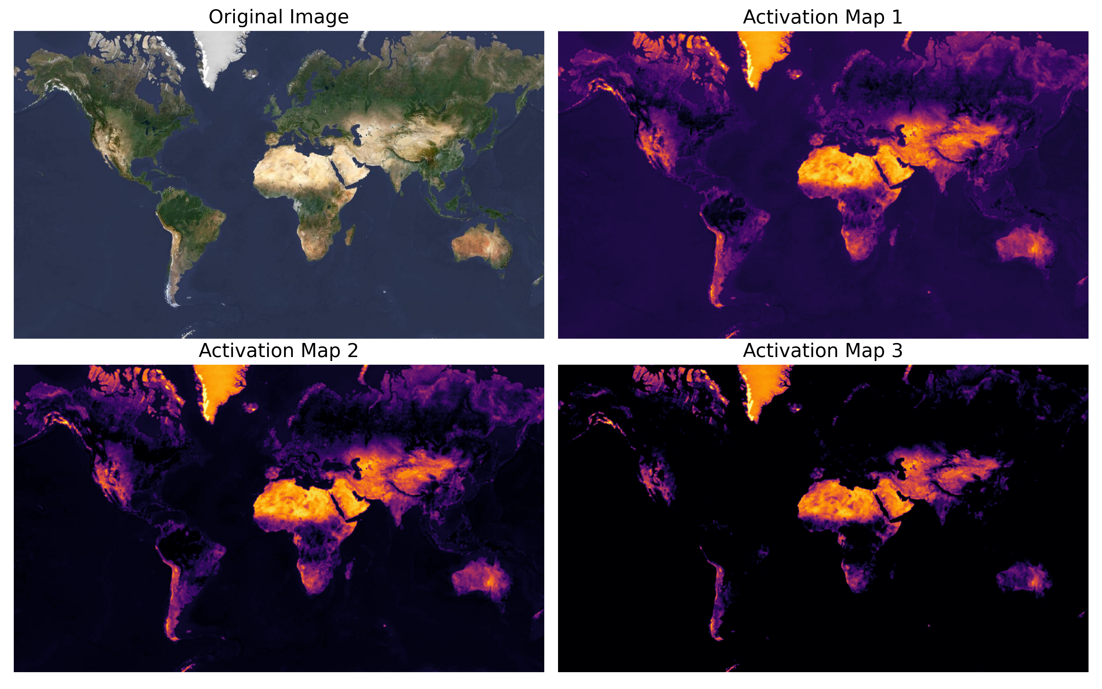
The MOSAIKS team performed a single featurization pass over the Planet Labs 2019 Q3 Visual Basemap images. The process is similar to the Random Convolutional Features (RCFs) method described earlier, but here are the specific parameters:
-
Patch Collection
- Random patches (filters) were drawn from real satellite images (Planet Labs 2019 Q3).
- Each patch was whitened: the raw pixel values were mean-centered and decorrelated so that each filter highlights distinct visual patterns.
- Random patches (filters) were drawn from real satellite images (Planet Labs 2019 Q3).
-
Kernel Sizes
-
2,000 features from a 4×4 patch shape
-
2,000 features from a 6×6 patch shape
- All patches maintain 3 color channels (R, G, B).
-
2,000 features from a 4×4 patch shape
-
Bias & Activation
- A bias of –1 is added to each filter’s convolution output, allowing more nuanced activation levels.
- A ReLU activation (
max(0, x)) is then applied to keep the model non-linear and remove negative values.
- A bias of –1 is added to each filter’s convolution output, allowing more nuanced activation levels.
-
Pooling
- After convolution + ReLU, the response is average-pooled over each 0.01° patch (i.e., the local 256×256 pixel area, if we approximate each degree of latitude or longitude as ~100 km—though the exact pixel count can vary by latitude).
- This results in a single numeric value per filter.
- After convolution + ReLU, the response is average-pooled over each 0.01° patch (i.e., the local 256×256 pixel area, if we approximate each degree of latitude or longitude as ~100 km—though the exact pixel count can vary by latitude).
-
Final Feature Vector
- Combining all filters yields a 4,000-dimensional vector at each 0.01° grid cell.
- This entire process was run once, creating a global 0.01° “feature layer.”
- Combining all filters yields a 4,000-dimensional vector at each 0.01° grid cell.
13.4 Derived aggregations
Although the API stores and provides these features at 0.01° resolution, it also offers pre-aggregated versions:
| Resolution | Description | Weighting | Download | Access |
|---|---|---|---|---|
| 0.01° | Native resolution (~1km²) | Unweighted | Map or File Query | API Portal |
| 0.1° | Aggregated grid (~10km²) | Area or population | Chunked files | Global Grids |
| 1° | Aggregated grid (~100km²) | Area or population | Single file | Global Grids |
| ADM2 | County or district level | Area or population | Single file | Precomputed Files |
| ADM1 | State or province level | Area or population | Single file | Precomputed Files |
| ADM0 | Country level | Area or population | Single file | Precomputed Files |
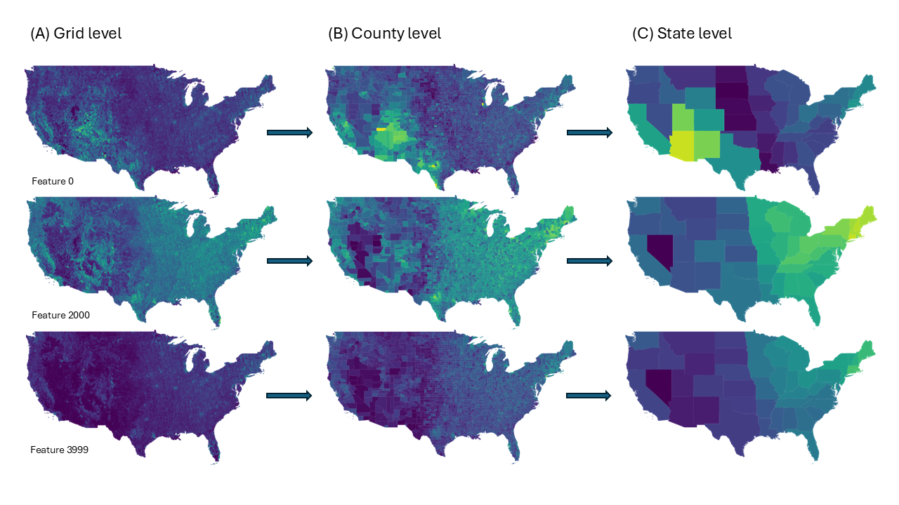
It is nice to have options, but sometimes it is hard to visualize what these aggregations mean. Figure 13.3 shows how these features might look when aggregated to different levels.
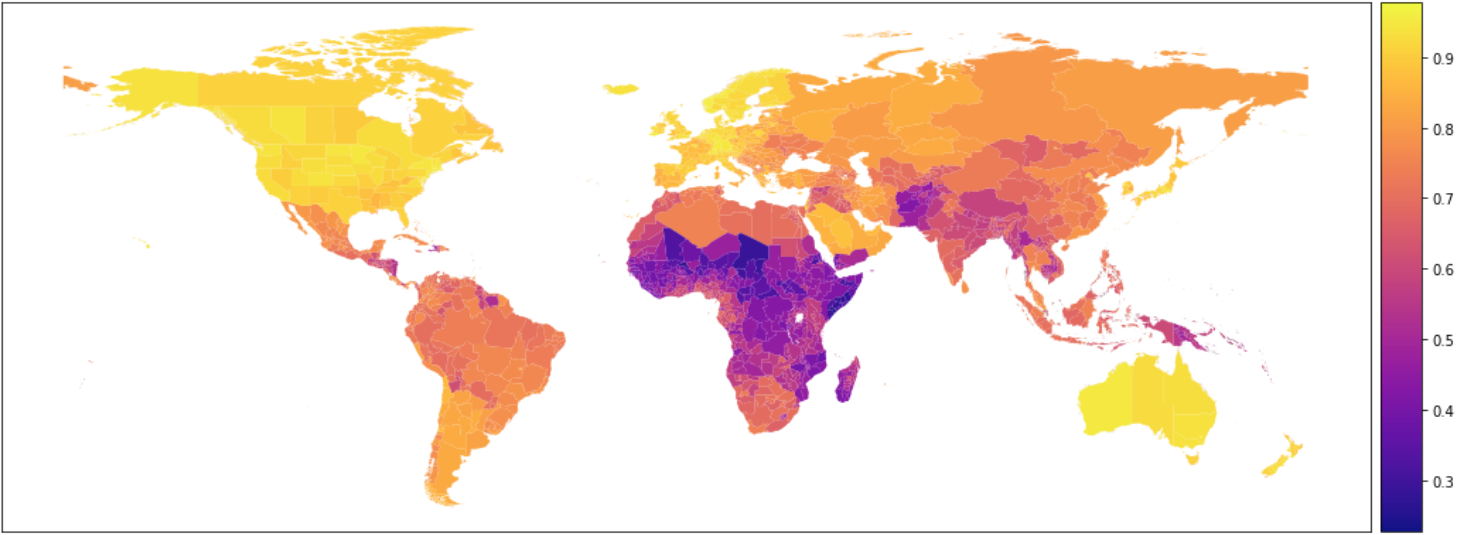
13.4.1 Area vs. Population Weighting
Each aggregated level comes in two weighting flavors: - Area Weighting: Larger grid cells or polygons with more land area receive more weight in the aggregation.
- Population Weighting: Uses population density (GPWv4) to weight cells more heavily where more people live.
note maybe a population map here
13.5 When to use these features
Readily Available: If your labels are from ~2019 or a period that hasn’t changed drastically since 2019, start with these API features—they’re the fastest and easiest to incorporate into your analyses.
Coarse-Resolution or Aggregated Labels: If your data is aggregated (e.g., a country-level statistic), consider downloading the aggregated features to match your label resolution.
Resource Constraints: If you’re storage- or compute-limited, using the API’s pre-aggregated files can save time and processing overhead.
High-Resolution or Household Data: For fine-grained tasks (e.g., household surveys), you may still benefit from the 0.01° resolution features—especially if you want to capture local variation. Or you can aggregate to match your label geometry and then use high-resolution features for prediction later (see Chapter 17).
13.6 Key takeaways
-
Single Source Imagery
-
Planet Labs Visual Basemap (2019 Q3)
- Global coverage of land areas at approximately 0.01° (~1 km) resolution
- Three color channels (Red, Green, Blue)
-
Planet Labs Visual Basemap (2019 Q3)
-
Single Featurization Pass
- All features are computed once at the native 0.01° resolution.
- Any aggregated features (e.g., 0.1°, 1°, administrative boundaries) are derivative and use exactly the same underlying 0.01° features.
- All features are computed once at the native 0.01° resolution.
-
Random Convolutional Features (RCFs)
-
4,000 total features
-
Kernel sizes: 2,000 features from a 4×4 kernel, and 2,000 features from a 6×6 kernel
-
Empirical patch whitening: random patches are drawn from the image set and then whitened (mean-centered, decorrelated)
-
Bias: –1 (applied to each filter output before activation)
-
Activation: ReLU (Rectified Linear Unit)
- 3 color channels from the original RGB imagery
-
4,000 total features
-
Flexible Resolutions
-
High resolution (0.01°): Download via File Query or Map Query
- Aggregations: 0.1°, 1°, and ADM0/ADM1/ADM2 boundaries, available as precomputed downloads
-
High resolution (0.01°): Download via File Query or Map Query
-
Use Cases
- Ideal for tasks with label data from the same (or close) time period (2019 or neighboring years)
- Quick, straightforward integration into machine learning models
- Global scale analysis or smaller local/regional analysis
- Ideal for tasks with label data from the same (or close) time period (2019 or neighboring years)
13.7 Future directions
In the next section, we will